Lecture 14: Quiz-I Discussion

IndiGo - a low-cost Indian airline company wants to introduce business class service on its domestic flight between Delhi and Mumbai. IndiGo’s operations research team predicts passenger demand (per trip) to follow a normal distribution with a mean of 10.35 and 155.25 passengers for business and economy class, respectively; and likewise, a standard deviation of 1 and 15 passengers for business and economy class, respectively. Notably, a row of business class includes 4 seats, wherein each seat takes up 5400 \(\text{cm}^2\), costs ₹15,000 to install, and earns a revenue of ₹20,000 per trip. On the other hand, a row of economy class includes 6 seats, wherein each seat takes up 3200 \(\text{cm}^2\), costs ₹5000 to install, and earns a revenue of ₹8000 per trip. To provide sufficient leg space, the total area covered by all seats should not exceed 72 \(\text{m}^2\). How many rows of business class (\(x_1\)) and economy class (\(x_2\)) should IndiGo configure in its Airbus A321neo airplane to ensure 95% service level, given that this airplane will make 6 trips per day between Delhi and Mumbai, every day for next 5 years? Assume a discount rate of 3%, and ignore all operational costs.

1. Objective Function

   1.1. Formulate net present value of IndiGo’s daily revenue (report the outcome in ₹abcd.e cr) (2)

   \[\begin{split} \begin{aligned} R_t & = (20,000 \times 10.35) + (8,000 \times 155.25) \times 6 \times 365 = 317.3 cr \\ \eta & = (1 - (1 + 0.03)^{-5}) / 0.03 = 4.58 \end{aligned} \end{split}\]

   Rendering, ₹\(1453.3 \text{cr} \ (1.453 \times 10^{10})\) in IndiGo’s revenue over the period of 5 years.

   
   

   1.2. Formulate IndiGo’s fixed cost. (1)

   \(FC = (15,000 \times 4)x_1 + (5,000 \times 6)x_2 = (6x_1 + 3x_2) \times 10^4\)

   
   

   1.3. Using above formulations, formulate IndiGo’s daily profit. (1)

   \(P = 1.4533 \times 10^{10} - (6x_1 + 3x_2) \times 10^4\)

   
   

2. Constraints

   2.1. Formulate all the technical constraints. (3)

   \[\begin{split} \begin{aligned} 4x_1 & \geq 10.35 + z_{0.95} \times 1; \ & x_1 & \geq 3 \\ 6x_2 & \geq 155.25 + z_{0.95} \times 15; \ & x_2 & \geq 30 \\ (0.54 \times 4)x_1 + (0.32 \times 6)x_2 & \leq 72; \ & 2.16x_1 + 1.92x_2 & \leq 72 \end{aligned} \end{split}\]
   
   

   2.2. Formulate all the domain constraints. (1)

   \(x_1, x_2 \in \mathbb{Z}_+\)

   
   

3. Formulation

   3.1. Formulate the problem as a standard linear programming model. (5)

   Objective:

   \[ \min_{x_1, x_2} \ z = (6x_1 + 3x_2) \times 10^4 \]

   Subject to:

   \[\begin{split} \begin{aligned} x_1 & \geq 3 \\ x_2 & \geq 30 \\ - 2.16x_1 - 1.92x_2 & \geq - 72 \\ x_1, x_2 & \in \mathbb{R}_+ \end{aligned} \end{split}\]
   
   

   3.3. Categorise the problem based on its functional, temporal, and certainty form. (3)

   Functional Form - Linear

   Temporal Form - Static

   Certainty Form - Stochastic

   
   

   3.3. State the necessary assumptions pertaining to the formulation. (2)

   Proportionaly, Additivity, Divisibility, and Certainty.

   
   

4. Graphical Solution Method (draw separate figures for each question below)

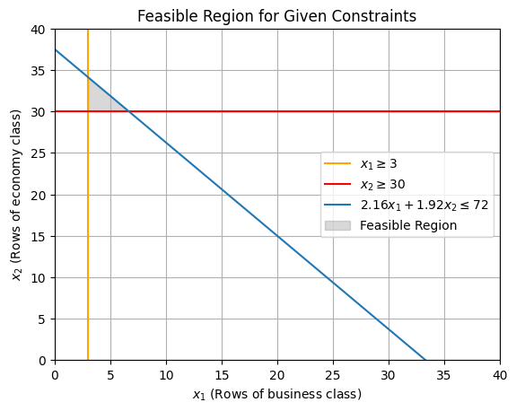
   4.1. Draw the feasible region. (4) (Label each constraint and clearly indicate the region that represents the feasible region)

import numpy as np
import matplotlib.pyplot as plt

# Define constraint coefficients
c1, c2 = 60000, 30000                 # Parameters for the objective function c1 * x1 + c2 * x2
a11, a12, b1 = 1, 0, 3                # Coefficients for constraint a11 * x1 + a12 * x2 >= b1
a21, a22, b2 = 0, 1, 30               # Coefficients for constraint a21 * x1 + a22 * x2 >= b2
a31, a32, b3 = 2.16, 1.92, 72         # Coefficients for constraint a31 * x1 + a32 * x2 <= b3

# Define the range of x1 values
x1 = np.linspace(0, 40, 400)

# Calculate x2 values for each constraint
x2_1 = np.full_like(x1, b1)   # From a11 * x1 + a12 * x2 >= b1
x2_2 = np.full_like(x1, b2)   # From a21 * x1 + a22 * x2 >= b2
x2_3 = (b3 - a31 * x1) / a32  # From a11 * a31 * x1 + a32 * x2 >= b3

# Plot the constraints
plt.axvline(x=b1, label=fr'$x_1 \geq {b1}$', color='orange')
plt.axhline(y=b2, label=fr'$x_2 \geq {b2}$', color='red')
plt.plot(x1, x2_3, label=fr'${a31}x_1 + {a32}x_2 \leq {b3}$')

# Fill the feasible region
plt.fill_between(x1, x2_2, np.maximum(x2_2, x2_3), where=(x1 >= x2_1), color='grey', alpha=0.3, label="Feasible Region")
                 
# Set plot attributes
plt.xlim(0, 40)
plt.ylim(0, 40)
plt.xlabel(r'$x_1$ (Rows of business class)')
plt.ylabel(r'$x_2$ (Rows of economy class)')
plt.legend()
plt.title("Feasible Region for Given Constraints")
plt.grid(True)

# Display the figure
plt.show()

4. Graphical Solution Method (draw separate figures for each question below)

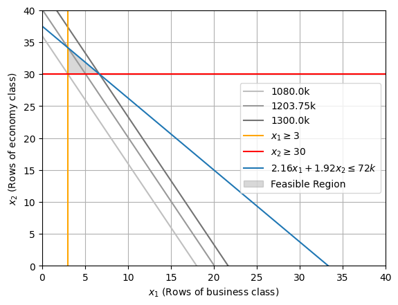
   4.2. Draw the iso-cost lines through each corner point of the feasible region. (3) (Redraw the feasible region and then draw the iso-cost lines; Label each constraint as well as the iso-cost lines).

import numpy as np
import matplotlib.pyplot as plt

# Define constraint coefficients
c1, c2 = 60000, 30000                 # Parameters for the objective function c1 * x1 + c2 * x2
a11, a12, b1 = 1, 0, 3                # Coefficients for constraint a11 * x1 + a12 * x2 >= b1
a21, a22, b2 = 0, 1, 30               # Coefficients for constraint a21 * x1 + a22 * x2 >= b2
a31, a32, b3 = 2.16, 1.92, 72         # Coefficients for constraint a31 * x1 + a32 * x2 <= b3

# Define set of isocost values (C)
C = [1080000, 1203750, 1300000]

for i,c in enumerate(C):
  # Calculate x2 value for iscost line c1 * x2 + c2 * x2 = c
  x2 = (c - c1 * x1) / c2
  # Plot the isocost lines
  plt.plot(x1, x2, color=str(0.75 - 0.15 * i), label=f'{c/1000}k')

# Define the range of x1 values
x1 = np.linspace(0, 40, 400)

# Calculate x2 values for each constraint
x2_1 = np.full_like(x1, b1)   # From a11 * x1 + a12 * x2 >= b1
x2_2 = np.full_like(x1, b2)   # From a21 * x1 + a22 * x2 >= b2
x2_3 = (b3 - a31 * x1) / a32  # From a11 * a31 * x1 + a32 * x2 >= b3

# Plot the constraints
plt.axvline(x=b1, label=fr'$x_1 \geq {b1}$', color='orange')
plt.axhline(y=b2, label=fr'$x_2 \geq {b2}$', color='red')
plt.plot(x1, x2_3, label=fr'${a31}x_1 + {a32}x_2 \leq {b3}k$')

# Fill the feasible region
plt.fill_between(x1, x2_2, np.maximum(x2_2, x2_3), where=(x1 >= x2_1), color='grey', alpha=0.3, label="Feasible Region")
                 
# Set plot attributes
plt.xlim(0, 40)
plt.ylim(0, 40)
plt.xlabel(r'$x_1$ (Rows of business class)')
plt.ylabel(r'$x_2$ (Rows of economy class)')
plt.legend()
plt.grid(True)

# Display the figure
plt.show()

4. Graphical Solution Method (draw separate figures for each question below)

   4.3. Report the optimal solution for the standardised linear programming model. (1)

   \(x_1, x_2 = 3, 30\)

   
   

   4.4. Classify each technical constraint as binding/non-binding. (1)

   Binding - \(x_1 \geq 3; \ x_2 \geq 30\)

   Non-binding - \(2.16x_1 + 1.92x_2 \leq 72\)

   
   

5. Solution Inference

   5.1. How many rows of business and economy class seats should IndiGo configure? (1)

   IndiGo should configure 3 rows of business class and 30 rows of economy class.

   
   

   5.1. Find the ratio of business to economy class seat installation cost \((c_1/c_2=r)\) that renders multiple optimal solutions? (1)

   No practical scenario would render multiple optimal solutions.

   
   

   5.2. For \(c_1/c_2=1\) how many rows of business and economy class seats should IndiGo configure? (1)

   IndiGo should configure 3 rows of business class and 30 rows of economy class.