
Lecture 9: Basic Linear Algebra#
Note
In this lecture, we will cover fundamental concepts in linear algebra to establish the foundation needed for understanding the Simplex Algorithm, which will be discussed in the next lecture.
Linear Algebra#
Matrices#
A matrix is a rectangular array of numbers with \(r\) rows and \(c\) columns, thus having a dimension of \(r \times c\).
For example,
Note, the element from \(i^{th}\) row and \(j^{th}\) column of matrix \(\mathbf{M}\) is given by \(m_{ij}\).
Vectors#
A vector is a one-dimensional matrix with an array of numbers arranged either in a column or in a row. Thus, a column vector with \(n\) rows has a dimension of \(n \times 1\), while a row vector with \(n\) columns has a dimension of \(1 \times n\).
For example,
Here, the \(i^{th}\) element of vector \(v\) is given by \(v_i\).
Note, any \(m\)-dimensional vector corresponds to a directed line segment in the \(m\)-dimensional plane.
Operations#
Addition
Two matrices - \(\mathbf{A}\) and \(\mathbf{B}\), with same dimension - \(r \times c\), can be summed up to render a resultant matrix - \(\mathbf{M}\), wherein the element from \(i^{th}\) row and \(j^{th}\) column is the sum of respective elements from the two matrices.
\[ m_{ij} = a_{ij} + b_{ij} \]Note, matrix addition holds:
Commutative Property: For any two matrices with same dimension, the order of addition does not affect the outcome.
\[ \mathbf{A} + \mathbf{B} = \mathbf{B} + \mathbf{A} \]Associative Property: For any three matrices with same dimension, the grouping of matrices does not affect the outcome.
\[ \mathbf{A} + (\mathbf{B} + \mathbf{C}) = (\mathbf{A} + \mathbf{B}) + \mathbf{C} \]Identity Property: For any matrix, there exists a zero matrix with the same dimension, such that,
\[ \mathbf{A} + \mathbf{O} = \mathbf{A} \]Inverse Property: For any matrix, there exists an inverse matrix with same dimension, such that,
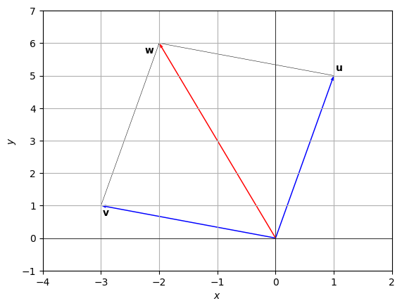
\[ \mathbf{A} + \mathbf{-A} = \mathbf{O} \]Below is a special case with 2-dimensional vectors \(u=[1,5]\) and \(v=[-3,1]\) summed in the 2-dimensional plane.
Multiplication
Scalar Product
The product of a constant \(n\) with matrix \(\mathbf{M}\) renders a matrix with elements of \(\mathbf{M}\) multiplied by \(n\).
\[ n\mathbf{M} = [nm_{ij}] \]Matrix Product
For two matrices - \(\mathbf{A}\) and \(\mathbf{B}\), their matrix product is only defined if the number of columns in \(\mathbf{A}\) equals the the number of rows in \(\mathbf{B}\). Thus, for such two matrices with dimension \(r_A \times n\) and \(n \times c_B\), respecitvely, the matrix product renders a \(r_A \times c_B\) matrix, wherein the \(ij^{th}\) element is the sum-product of elements from row \(i\) of matrix \(\mathbf{A}\) and column \(j\) of matrix \(\mathbf{B}\).
\[ \mathbf{A} \times \mathbf{B} = [\sum_{k \in n} a_{ik}b_{kj}]_{r_A \times c_B} \]Note, matrix multiplication holds
Non-Commutative Property: For any two matrices, the order of multiplication affects the outcome.
\[ \mathbf{A} \mathbf{B} \ne \mathbf{B} \mathbf{A} \]Associative Property: For any three matrices with compatible dimensions, the grouping of matrices does not affect the outcome.
\[ \mathbf{A} (\mathbf{B} \mathbf{C}) = (\mathbf{A} \mathbf{B}) \mathbf{C} \]Distributive Property: For any three matrices with compatible dimensions, multiplication is ditributive over addition.
\[ \mathbf{A} (\mathbf{B} + \mathbf{C}) = (\mathbf{A} + \mathbf{B}) \mathbf{C} \]Identity Property: For any matrix, there exists an identity matrix with the same dimension, such that,
\[ \mathbf{A} \mathbf{I} = \mathbf{A} \]Transpose
Given a matrix \(\mathbf{M} = [m_{ij}]\) with \(r\) rows and \(c\) columns, then the transpose matrix is a \(c \times r\) matrix such that \(\mathbf{M}^T = [m_{ji}]\)
Note, matrix transpose holds
Distributive Property: For any two matrices with compatible dimensions, transpose is ditributive over addition and reverse distributive over multiplication.
\[ (\mathbf{A} + \mathbf{B}) ^ T = \mathbf{A} ^ T + \mathbf{B} ^ T \]\[ (\mathbf{A} \mathbf{B}) ^ T = \mathbf{B} ^ T \mathbf{A} ^ T \]Inverse
Given a square matrix \(\mathbf{M}\) with \(n\) rows and \(n\) columns, the inverse matrix \(\mathbf{M}^{-1}\) satisfies \(\mathbf{M}\mathbf{M}^{-1} = \mathbf{I}_n\), where \(\mathbf{I}_n\) is an \(n \times n\) identity matrix.
Finding Inverse of a Matrix
Procedural
Let,
\[\begin{split} \mathbf{M} = \begin{bmatrix} 2 & 0 & -1 \\ 3 & 1 & 2 \\ -1 & 0 & 1 \end{bmatrix} \end{split}\]We have,
\[ \mathbf{M}\mathbf{M}^{-1} = \mathbf{I}_n \]\[\begin{split} \begin{bmatrix} 2 & 0 & -1 \\ 3 & 1 & 2 \\ -1 & 0 & 1 \end{bmatrix} \mathbf{M}^{-1} = \begin{bmatrix} 1 & 0 & 0 \\ 0 & 1 & 0 \\ 0 & 0 & 1 \end{bmatrix} \end{split}\]Transform \(\mathbf{M}\) into \(\mathbf{I}_n\) and make equivalent transformations to \(\mathbf{I}_n\)
The general transformation process involves iterating over each row, each column, and transforming every non-diagonal element to 0, albeit not necessarily in a chronological manner. Here after, iterate over each row, each column, transforming every diagonal element to 1.
\[ r_1 \gets r_1 + r_3 \]\[\begin{split} \begin{bmatrix} 1 & 0 & 0 \\ 3 & 1 & 2 \\ -1 & 0 & 1 \end{bmatrix} \mathbf{M}^{-1} = \begin{bmatrix} 1 & 0 & 1 \\ 0 & 1 & 0 \\ 0 & 0 & 1 \end{bmatrix} \end{split}\]\[ r_2 \gets r_2 + 3r_3 \]\[\begin{split} \begin{bmatrix} 1 & 0 & 0 \\ 0 & 1 & 5 \\ -1 & 0 & 1 \end{bmatrix} \mathbf{M}^{-1} = \begin{bmatrix} 1 & 0 & 1 \\ 0 & 1 & 3 \\ 0 & 0 & 1 \end{bmatrix} \end{split}\]\[ r_3 \gets r_3 + r_1 \]\[\begin{split} \begin{bmatrix} 1 & 0 & 0 \\ 0 & 1 & 5 \\ 0 & 0 & 1 \end{bmatrix} \mathbf{M}^{-1} = \begin{bmatrix} 1 & 0 & 1 \\ 0 & 1 & 3 \\ 1 & 0 & 2 \end{bmatrix} \end{split}\]\[ r_2 \gets r_2 - 5r_3 \]\[\begin{split} \begin{bmatrix} 1 & 0 & 0 \\ 0 & 1 & 0 \\ 0 & 0 & 1 \end{bmatrix} \mathbf{M}^{-1} = \begin{bmatrix} 1 & 0 & 1 \\ -5 & 1 & -7 \\ 1 & 0 & 2 \end{bmatrix} \end{split}\]\[\begin{split} r_1 \gets r_1/1 \\ r_2 \gets r_2/1 \\ r_3 \gets r_3/1 \\ \end{split}\]\[\begin{split} \begin{bmatrix} 1 & 0 & 0 \\ 0 & 1 & 0 \\ 0 & 0 & 1 \end{bmatrix} \mathbf{M}^{-1} = \begin{bmatrix} 1 & 0 & 1 \\ -5 & 1 & -7 \\ 1 & 0 & 2 \end{bmatrix} \end{split}\]Thus,
\[\begin{split} \mathbf{M^{-1}} = \begin{bmatrix} 1 & 0 & 1 \\ -5 & 1 & -7 \\ 1 & 0 & 2 \end{bmatrix} \end{split}\]Formulaic
\[\begin{split} \mathbf{M^{-1}} = 1 / |\mathbf{M}| \begin{bmatrix} |\mathbf{M}^{11}| & |\mathbf{M}^{12}| & \cdots & |\mathbf{M}^{1c}| \\ |\mathbf{M}^{21}| & |\mathbf{M}^{22}| & \cdots & |\mathbf{M}^{2c}| \\ \vdots & \vdots & \ddots & \vdots \\ |\mathbf{M}^{r1}| & |\mathbf{M}^{r2}| & \cdots & |\mathbf{M}^{rc}| \end{bmatrix} \end{split}\]Where, \(\mathbf{M}^{ij} = [m_{kl}; m_{kl} \in \mathbf{M}, k \ne i, l \ne j]\), i.e., \(\mathbf{M}^{ij}\) is a matrix with elements from \(\mathbf{M}\) exlucding row \(i\) and column \(j\).
Notice that the inverse will only exist if the determinant is non-zero!
import numpy as np

A = np.matrix('2, 0, -1; 3, 1, 2; -1, 0, 1')
B = np.linalg.inv(A)

print(B)
[[ 1.  0.  1.]
 [-5.  1. -7.]
 [ 1.  0.  2.]]
System of Equations#
Consider a set of linear equations given by,
Here, \(x_i\) are variables, while \(a_{ij}\) and \({b_i}\) are referred to as parameters.
These set of linear equations can be represented in matrix form as,
Where,
Thus,
Note, here \(\mathbf{x}\) exists if and only if inverse of \(\mathbf{A}\) exists, i.e., if \(\mathbf{A}\) is a square matrix with non-zero determinant.
Note
In the next few lectures, we will apply the concepts of linear algebra discussed in this lecture, to solve the linear optimisation problems using the Simplex Algorithm.