
Lecture 11: Sensitivity Analysis#
Note
Having solved linear optimization problems, this lecture will focus on Sensitivity Analysis—examining how changes in parameter values impact the optimal solution and the resulting optimal value.
Example#
Consider a textile firm operating in Kochi. This company needs to ship 100 tons of textile goods from Kanchipuram and can rent two types of trucks - \(\text{T}_1\) and \(\text{T}_2\). Each truck of type \(\text{T}_1\) can carry 10 tons of goods and costs ₹5000 per trip, while each truck of type \(\text{T}_2\) can carry 20 tons and costs ₹8000 per trip. Further, considering the managerial capacity of the firm (warehouse capacity, staff numbers, etc.), the management committee has imposed an upper limit on truck rental of 20 trucks in total, with a maximum of 12 any individual type of truck. Thus, how many \(\text{T}_1\) and \(\text{T}_2\) type trucks should the company deploy so as to minimize the total costs?
Subject to:
Caution
For representation purpose, we have relaxed the constraint \(x_1, x_2 \in \mathbb{Z}_+\) to \(x_1, x_2 \geq 0\) in the above formulation.
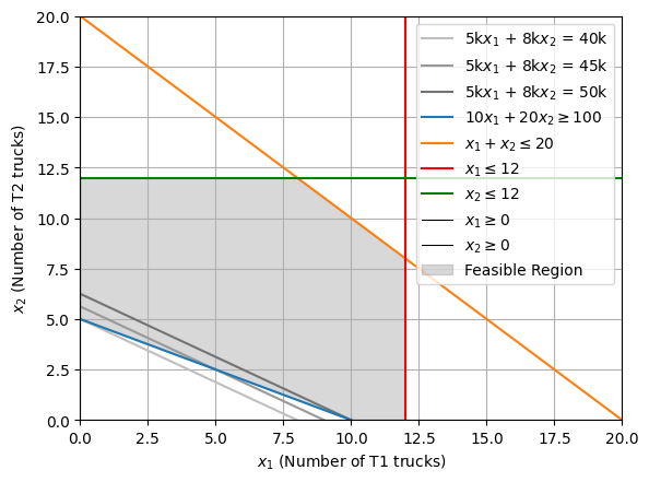
The corner point, \((0,5)\) is the optimal solution, thus implying that the firm should purchase 5 \(\text{T}_2\) type trucks to ship 100 tons of textile goods from Kanchipuram to Kochi, amounting to a total cost of ₹40k.
Cost Sensitivity#
How does varying \(\text{T}_2\)’s shipping cost impact the optimal solution?
import numpy as np
import ipywidgets as widgets
import matplotlib.pyplot as plt

# Define objective function parameters and constraint coefficients
c1, c2 = 5000, 8000         # Parameters for the objective function c1 * x1 + c2 * x2
a11, a12, b1 = 10, 20, 100  # Coefficients for constraint a11 * x1 + a12 * x2 >= b1
a21, a22, b2 = 1, 1, 20     # Coefficients for constraint a21 * x1 + a22 * x2 <= b2
a31, a32, b3 = 1, 0, 12     # Coefficients for constraint a31 * x1 + a32 * x2 <= b3
a41, a42, b4 = 0, 1, 12     # Coefficients for constraint a41 * x1 + a42 * x2 <= b4

def slide(c2):
  # Define the range of x1 values
  x1 = np.linspace(0, max(b1/a11, b2/a21, b3/a31), 400)

  # Define set of isocost values (C)
  C = [40000, 50000, 60000]

  for i,c in enumerate(C):
    # Calculate x2 value for isocost line c1 * x1 + c2 * x2 = c
    x2 = (c - c1 * x1) / c2
    # Plot the isocost lines
    plt.plot(x1, x2, color=str(0.75 - 0.15 * i), label=f'{c1//1000}k$x_1$ + {c2//1000}k$x_2$ = {c//1000}k')

  # Calculate x2 values for each constraint
  x2_1 = (b1 - a11 * x1) / a12  # From a11 * x1 + a12 * x2 >= b1
  x2_2 = (b2 - a21 * x1) / a22  # From a21 * x1 + a22 * x2 <= b2
  x2_3 = np.full_like(x1, b3)   # From a31 * x1 + a32 * x3 <= b3
  x2_4 = np.full_like(x1, b4)   # From a41 * x1 + a42 * x4 <= b4

  # Plot the constraints
  plt.plot(x1, x2_1, label=fr'${a11}x_1 + {a12}x_2 \geq {b1}$')
  plt.plot(x1, x2_2, label=fr'$x_1 + x_2 \leq {b2}$')
  plt.axvline(x=b3, label=fr'$x_1 \leq {b3}$', color='red')
  plt.axhline(y=b4, label=fr'$x_2 \leq {b4}$', color='green')
  plt.axvline(x=0, label=fr'$x_1 \geq 0$', color='black', linewidth=0.75)
  plt.axhline(y=0, label=fr'$x_2 \geq 0$', color='black', linewidth=0.75)

  # Fill the feasible region where all constraints are satisfied
  plt.fill_between(x1, np.maximum(x2_1, 0), np.maximum(np.maximum(x2_1, 0), np.minimum(x2_2, x2_4)), where=(x1 <= x2_3) & (x1 >= 0), color='grey', alpha=0.3, label="Feasible Region")

  # Set plot attributes
  plt.xlim(0, max(b1/a11, b2/a21, b3))
  plt.ylim(0, max(b1/a12, b2/a22, b4))
  plt.xlabel(r'$x_1$ (Number of T1 trucks)')
  plt.ylabel(r'$x_2$ (Number of T2 trucks)')
  plt.legend()
  plt.grid(True)

  # Display the plot
  plt.show()

widgets.interact(slide, c2=widgets.IntSlider(value=8000, min=8000, max=12000, step=100, description=r'T2 shipping cost (₹/km)'))
<function __main__.slide(c2)>
Thus, if \(\text{T}_1\)’s shipping cost (\(c_1\)) and \(\text{T}_2\)’s shipping cost (\(c_2\)) is such that \(c_1 / c_2 = 0.5\), then all combinations that satisfy \(10x_1 + 20x_2 = 100\) are optimal. Specifically, the firm can purhcase any of the following combinations,
# \(\text{T}_1\) Trucks |
# \(\text{T}_2\) trucks |
|---|---|
10 |
0 |
8 |
1 |
6 |
2 |
4 |
3 |
2 |
4 |
0 |
5 |
However, if \(c_1 / c_2 > 0.5\), then the firm should purchase 5 \(\text{T}_2\) type trucks to ship goods from Kanchipuram to Kochi. On the other hand, if \(c_1 / c_2 < 0.5\), then the firm should purchase 10 \(\text{T}_1\) type trucks.
Caution
The inference here is only valid holding other parameter values fixed, i.e., for the given values of shipment demand, truck capacity, and fleet size limit.
Capacity Sensitivity#
How does varying \(\text{T}_1\)’s capacity impact the optimal solution?
import numpy as np
import ipywidgets as widgets
import matplotlib.pyplot as plt

# Define objective function parameters and constraint coefficients
c1, c2 = 5000, 8000         # Parameters for the objective function c1 * x1 + c2 * x2
a11, a12, b1 = 10, 20, 100  # Coefficients for constraint a11 * x1 + a12 * x2 >= b1
a21, a22, b2 = 1, 1, 20     # Coefficients for constraint a21 * x1 + a22 * x2 <= b2
a31, a32, b3 = 1, 0, 12     # Coefficients for constraint a31 * x1 + a32 * x2 <= b3
a41, a42, b4 = 0, 1, 12     # Coefficients for constraint a41 * x1 + a42 * x2 <= b4

def slide(a11):
  # Define the range of x1 values
  x1 = np.linspace(0, max(b1/a11, b2/a21, b3/a31), 400)

  # Define set of isocost values (C)
  C = [30000, 40000, 50000]

  for i,c in enumerate(C):
    # Calculate x2 value for isocost line c1 * x1 + c2 * x2 = c
    x2 = (c - c1 * x1) / c2
    # Plot the isocost lines
    plt.plot(x1, x2, color=str(0.75 - 0.15 * i), label=f'{c1//1000}k$x_1$ + {c2//1000}k$x_2$ = {c//1000}k')

  # Calculate x2 values for each constraint
  x2_1 = (b1 - a11 * x1) / a12  # From a11 * x1 + a12 * x2 >= b1
  x2_2 = (b2 - a21 * x1) / a22  # From a21 * x1 + a22 * x2 <= b2
  x2_3 = np.full_like(x1, b3)   # From a31 * x1 + a32 * x3 <= b3
  x2_4 = np.full_like(x1, b4)   # From a41 * x1 + a42 * x4 <= b4

  # Plot the constraints
  plt.plot(x1, x2_1, label=fr'${a11}x_1 + {a12}x_2 \geq {b1}$')
  plt.plot(x1, x2_2, label=fr'$x_1 + x_2 \leq {b2}$')
  plt.axvline(x=b3, label=fr'$x_1 \leq {b3}$', color='red')
  plt.axhline(y=b4, label=fr'$x_2 \leq {b4}$', color='green')
  plt.axvline(x=0, label=fr'$x_1 \geq 0$', color='black', linewidth=0.75)
  plt.axhline(y=0, label=fr'$x_2 \geq 0$', color='black', linewidth=0.75)

  # Fill the feasible region where all constraints are satisfied
  plt.fill_between(x1, np.maximum(x2_1, 0), np.maximum(np.maximum(x2_1, 0), np.minimum(x2_2, x2_4)), where=(x1 <= x2_3) & (x1 >= 0), color='grey', alpha=0.3, label="Feasible Region")

  # Set plot attributes
  plt.xlim(0, max(b1/a11, b2/a21, b3))
  plt.ylim(0, max(b1/a12, b2/a22, b4))
  plt.xlabel(r'$x_1$ (Number of T1 trucks)')
  plt.ylabel(r'$x_2$ (Number of T2 trucks)')
  plt.legend()
  plt.grid(True)

  # Display the plot
  plt.show()

widgets.interact(slide, a11=widgets.IntSlider(value=10, min=10, max=15, step=1, description=r'T_1 capacity (tons)'))
Thus, if the capacity of \(\text{T}_1\) truck (\(q\)) is such that \(q/20 = 0.625\), then all values that satisfy on \(qx_1 + 20x_2 = 100\) are optimal. However, if \(q/20 > 0.625\), then the firm should purchase \(100 / q\) \(\text{T}_1\) type trucks. On the other hand, if \(q / 20 < 0.625\), then the firm should instead purchase 5 \(\text{T}_2\) type trucks to ship textile goods from Kachipuram to Kochi.
Caution
The inference here is only valid holding other parameter values fixed, i.e., for the given values of shipment demand, truck cost, and fleet size limit.
Demand Sensitivity#
How does varying shipment demand impact optimal solution?
import numpy as np
import ipywidgets as widgets
import matplotlib.pyplot as plt

# Define objective function parameters and constraint coefficients
c1, c2 = 5000, 8000         # Parameters for the objective function c1 * x1 + c2 * x2
a11, a12, b1 = 10, 20, 100  # Coefficients for constraint a11 * x1 + a12 * x2 >= b1
a21, a22, b2 = 1, 1, 20     # Coefficients for constraint a21 * x1 + a22 * x2 <= b2
a31, a32, b3 = 1, 0, 12     # Coefficients for constraint a31 * x1 + a32 * x2 <= b3
a41, a42, b4 = 0, 1, 12     # Coefficients for constraint a41 * x1 + a42 * x2 <= b4

def slide(b1):
  # Define the range of x1 values
  x1 = np.linspace(0, max(b1/a11, b2/a21, b3/a31), 400)

  # Define set of isocost values (C)
  C = [16000, 32000, 48000, 64000, 80000]

  for i,c in enumerate(C):
    # Calculate x2 value for isocost line c1 * x1 + c2 * x2 = c
    x2 = (c - c1 * x1) / c2
    # Plot the isocost lines
    plt.plot(x1, x2, color=str(0.75 - 0.15 * i), label=f'{c1//1000}k$x_1$ + {c2//1000}k$x_2$ = {c//1000}k')

  # Calculate x2 values for each constraint
  x2_1 = (b1 - a11 * x1) / a12  # From a11 * x1 + a12 * x2 >= b1
  x2_2 = (b2 - a21 * x1) / a22  # From a21 * x1 + a22 * x2 <= b2
  x2_3 = np.full_like(x1, b3)   # From a31 * x1 + a32 * x3 <= b3
  x2_4 = np.full_like(x1, b4)   # From a41 * x1 + a42 * x4 <= b4

  # Plot the constraints
  plt.plot(x1, x2_1, label=fr'${a11}x_1 + {a12}x_2 \geq {b1}$')
  plt.plot(x1, x2_2, label=fr'$x_1 + x_2 \leq {b2}$')
  plt.axvline(x=b3, label=fr'$x_1 \leq {b3}$', color='red')
  plt.axhline(y=b4, label=fr'$x_2 \leq {b4}$', color='green')
  plt.axvline(x=0, label=fr'$x_1 \geq 0$', color='black', linewidth=0.75)
  plt.axhline(y=0, label=fr'$x_2 \geq 0$', color='black', linewidth=0.75)

  # Fill the feasible region where all constraints are satisfied
  plt.fill_between(x1, np.maximum(x2_1, 0), np.maximum(np.maximum(x2_1, 0), np.minimum(x2_2, x2_4)), where=(x1 <= x2_3) & (x1 >= 0), color='grey', alpha=0.3, label="Feasible Region")

  # Set plot attributes
  plt.xlim(0, max(b2/a21, b3))
  plt.ylim(0, max(b2/a22, b4))
  plt.xlabel(r'$x_1$ (Number of T1 trucks)')
  plt.ylabel(r'$x_2$ (Number of T2 trucks)')
  plt.legend()
  plt.grid(True)

  # Display the plot
  plt.show()

widgets.interact(slide, b1=widgets.IntSlider(value=100, min=10, max=400, step=1, description=r'Shipment demand (tons)'))
Thus, if shipment demand is \(b_1 \text{tons}\) such that \(b_1 < 240\), then the firm should purchase \(b_1 / 20\) \(\text{T}_2\) type trucks to ship textile goods from Kachipuram to Kochi, rendering a total cost of ₹\(400 \times b_1\). However, if \(b_1 \in [240,320]\), then the firm should purchase 12 \(\text{T}_2\) type trucks and remaining \((b_1 - 240)/10\) \(\text{T}_1\) type trucks, resulting in a total cost of ₹\(500 \times b_1 -\) ₹\(24000\). Note, if \(b_1 > 320\), then an optimal solution does not exist for the problem.
Now then, increasing shipment demand by one unit will result in an increase in cost by ₹400 if \(b_1 < 240\), and ₹500 if \(b_1 \in [240,320]\). This is referred to as the shadow price, i.e, the change in objective function value if a constraint is relaxed/tightened by one unit.
Caution
The inference here is only valid holding other parameter values fixed, i.e., for the given values of truck capacity, truck cost, and fleet size limit.
Tip
Since binding constraints define the solution, only binding constraints have non-zero shadow price, while non-binding constraints have zero shadow price.