Lecture 5: Graphical Solution Method

Note

In this lecture, we will discuss the graphical solution method for linear programming through a two-variable problem.

---

Example #1

Consider a textile firm operating in Kochi. This company needs to ship 100 tons of textile goods from Kanchipuram and can rent two types of trucks - \(\text{T}_1\) and \(\text{T}_2\). Each truck of type \(\text{T}_1\) can carry 10 tons of goods and costs ₹5000 per trip, while each truck of type \(\text{T}_2\) can carry 20 tons and costs ₹8000 per trip. Thus, how many \(\text{T}_1\) and \(\text{T}_2\) type trucks should the company deploy so as to minimize the total costs?

Objective:

\[ \min_{x_1, x_2} \ z = 5000x_1 + 8000x_2 \]

Subject to:

\[\begin{split} \begin{aligned} 10x_1 + 20x_2 & \geq 100 \\ x_1, x_2 & \in \mathbb{Z}_+ \end{aligned} \end{split}\]

---

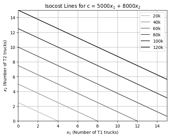
Iso-cost/Iso-profit curve

An iso-cost/iso-profit curve represents set of values for decision variables that yield the samle value for total cost/profit. Hence, for the example problem, the iso-cost lines are given by,

\[ c = 5000x_1 + 8000x_2 \]

---

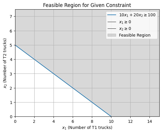
Feasible Region

Caution

For representation purpose, we have relaxed the constraint \(x_1, x_2 \in \mathbb{Z}_+\) to \(x_1, x_2 \geq 0\) in the following formulations.

The set of values of the decision variables that satisfy all given constraints constitute the feasible region. Any value within this region is thus referred to as a feasible value. Hence, for the example problem, the feasible region is defined by,

\[\begin{split} \begin{aligned} 10x_1 + 20x_2 & \geq 100 \\ x_1, x_2 & \geq 0 \end{aligned} \end{split}\]

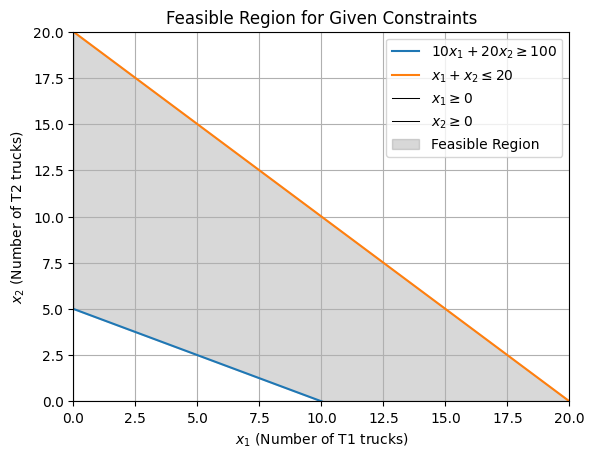
Considering the managerial capacity of the firm (warehouse capacity, staff numbers, etc.), the management committee has imposed an upper limit on truck rental of 20 trucks.

\[\begin{split} \begin{aligned} 10x_1 + 20x_2 & \geq 100 \\ x_1 + x_2 & \leq 20 \\ x_1, x_2 & \geq 0 \end{aligned} \end{split}\]

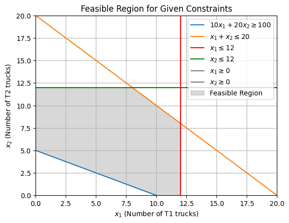
Considering the managerial capacity of the firm (warehouse capacity, staff numbers, etc.), the management committee has imposed an upper limit on truck rental of 20 trucks in total, with a maximum of 12 any individual type of truck.

\[\begin{split} \begin{aligned} 10x_1 + 20x_2 & \geq 100 \\ x_1 + x_2 & \leq 20 \\ x_1 & \leq 12 \\ x_2 & \leq 12 \\ x_1, x_2 & \geq 0 \end{aligned} \end{split}\]

The feasible regions discussed in this lecture can be referred to as bounded feasible regions. To be precise, bounded feasible region is one where all solutions are contained within a finite area, meaning the feasible region does not extend infinitely in any direction. On the other hand, an unbounded feasible region is one where the feasible region extends infinitely in at least one direction. We shall see such feasible regions in the next lecture.

---

Optimal Value

The feasible value that optimises (maximises/minimises) the objective function is called the optimal value. Thus, for the example problem,

Objective:

\[ \min_{x_1, x_2} \ z = 5000x_1 + 8000x_2 \]

Subject to:

\[\begin{split} \begin{aligned} 10x_1 + 20x_2 & \geq 100 \\ x_1, x_2 & \geq 0 \end{aligned} \end{split}\]

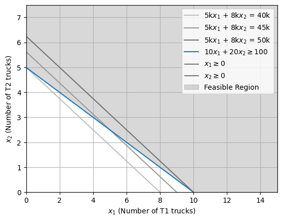
Notice, the solution of a linear programming problem will always lie at one of the corners of the feasible region due to proportionality property of linear problems. For the given problem, \((0,5)\) is the optimal solution, and hence, the textile firm should buy 5 \(\text{T}_2\) type trucks to ship cargo from Kanchipuram to Kochi, amounting to a total cost of ₹40k.

Now then, for,

Objective:

\[ \min_{x_1, x_2} \ z = 5000x_1 + 8000x_2 \]

Subject to:

\[\begin{split} \begin{aligned} 10x_1 + 20x_2 & \geq 100 \\ x_1 + x_2 & \leq 20 \\ x_1 & \leq 12 \\ x_2 & \leq 12 \\ x_1, x_2 & \geq 0 \end{aligned} \end{split}\]

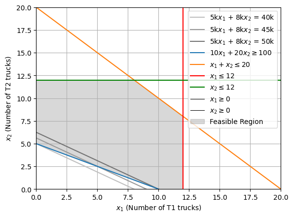
Here again, the corner point, \((0,5)\) is the optimal solution. Notice, constraints \(10x_1 + 20x_2 \geq 100\) and \(x_1 \geq 0\) define the solution, and thus are binding, while none of the other constraints shape the solution, and hence are non-binding. To be precise, a binding constraint is one that directly affects the optimal solution. At the optimal point, the constraint equation is exactly satisfied (meaning it “binds” or restricts the solution to that specific boundary). If this constraint were removed or relaxed, the optimal solution would change. On the other hand, a non-binding constraint is one that does not limit or affect the optimal solution. If this constraint were removed, the optimal solution would remain the same.

Now then, what if instead of a maximum of 12 \(\text{T}_2\) trucks, the manegerial committee had imposed a thershold of 4 trucks.

Objective:

\[ \min_{x_1, x_2} \ z = 5000x_1 + 8000x_2 \]

Subject to:

\[\begin{split} \begin{aligned} 10x_1 + 20x_2 & \geq 100 \\ x_1 + x_2 & \leq 20 \\ x_1 & \leq 12 \\ x_2 & \leq 4 \\ x_1, x_2 & \geq 0 \end{aligned} \end{split}\]

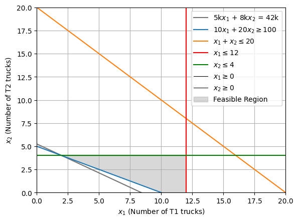
For the given problem, the corner point, \((2,4)\) is the optimal solution since constraints \(10x_1 + 20x_2 \geq 100\) and \(x_2 \geq 4\) are binding, while \(x_1 + x_2 \leq 20\) and \(x_1 \geq 12\) are non-binding. Thus, the textile firm should buy 2 \(\text{T}_2\) type trucks and 4 \(\text{T}_2\) type trucks to ship cargo from Kanchipuram to Kochi, amounting to a total cost of ₹42k.

---

Caution

The problems discussed in this lecture have a single optimal solution, however, a linear programming problem can have multiple optimal solutions if the objective function is parallel to a binding constraint within the feasible region, thus resulting in a line segment of optimal solutions rather than a single corner point. Nonetheless, a linear programming problem can also have no feasible solution if the constraints cannot collectively form a feasible region, making it impossible to satisfy all constraints simultaneously. We shall discuss such cases in the next lecture.