
Lecture 10: Simplex Method#
Note
In lecture 6, we employed graphical solution methods to solve two-variable linear optimisation problems. However, as discussed in lectures 7 and 8, a general \(n\)-dimensional problem requires more sophisticated computational tools. In the backend of these computational tools resides the Simplex Algorithm. In this lecture we will take a closer look at this algorithm to address general \(n\)-dimensional linear optimisation problems.
Recall, a typical linear optimisation problem can be expressed as,
Objective:
Subject to:
Here, \(f(\mathbf{x})\) is the objective function, \(x_i\) is a decision variable, \(a_{i1}x_1 + a_{i2}x_2 + ... + a_{in}x_n \geq b_i\) is a technical constraint, and \(x_i \geq 0\) is a domain constriant.
Note, an inequality constraint with \(a_{i1}x_1 + a_{i2}x_2 + ... + a_{in}x_n \leq 0\) can be re-written in the standard form as \(- a_{i1}x_1 - a_{i2}x_2 - ... - a_{in}x_n \geq 0\), while an equality constraint \(a_{i1}x_1 + a_{i2}x_2 + ... + a_{in}x_n = 0\) can be re-written in the standarad form as \(a_{i1}x_1 + a_{i2}x_2 + ... + a_{in}x_n \geq 0\); \(- a_{i1}x_1 - a_{i2}x_2 - ... - a_{in}x_n \geq 0\).
We will now transform the technical constraints into a system of equations by introducing a slack term into each constraint. Thus, we have the standardised form,
Objective:
Subject to:
The above formulation can now be represented in matrix form as,
Objective:
Subject to:
Where,
Now then, recall that we can solve the system of linear equations with,
However, \(\mathbf{x}\) exists if and only if inverse of \(\mathbf{A}\) exists, i.e., if \(\mathbf{A}\) is a square matrix with non-zero determinant. However, there is no reason for us to assume these conditions to hold true. Specifically, it is possible to have a linear optimisation problem with \(n\) decision variables and \(m\) constraints, rendering a rectangular matrix \(\mathbf{A}\) with \(m\) rows and \(n\) columns, where \(n \ne m\).
Now then, having converted the linear optimisation problem into a standardised form with \(n + m\) variables (\(n\) decision and \(m\) slack variables), we will now set \(n\) variables to 0 (referred to as non-basic variables; NBV), allowing us to uniquely compute the values for the remaining \((n + m) - n = m\) variables (referred to as basic variables; BV). If the resulting values of basic variables satisfy \(\mathbf{x,s} \geq 0\), then the set of basic and non-basic variable values together \((\mathbf{x,s})\) are said to form a basic feasible solution (BFS). For all such basic feasible solutions, we shall compute the objective function value and thus determine the optimal solution. This is the Simplex Algorithm.
Note, this process is equivalent evaluating all corner point solutions, computing the objective function value for each, and consequently determining the optimal solution. Through the following two-variable problem, we shall see that the basic feasible solutions are equivalent to the corner point solutions.
Objective:
Subject to:
We begin by transforming the maximisation problem into a typical minimisation problem.
Objective:
Subject to:
We will now transform the above formulation into the standardised form by introducing a slack term into the technical constraints.
Objective:
Subject to:
Here, we have a system of equations with 4 variables (2 decision and 2 slack variables). Hence, we shall set values for 2 non-basic variables as 0 and consequently evaluate values for remaining 2 basic variables.
Non-Basic Variables |
Basic Variables |
Decision Variable \(\\(x_1, x_2)\) |
Slack Variable \(\\(s_1, s_2)\) |
Is Basic Feasible Solution? |
|---|---|---|---|---|
\(x_1, x_2\) |
\(s_1, s_2\) |
0, 0 |
40, 60 |
Yes |
\(x_1, s_1\) |
\(x_2, s_2\) |
0, 40 |
0, 20 |
Yes |
\(x_1, s_2\) |
\(x_2, s_1\) |
0, 60 |
-20, 0 |
No |
\(x_2, s_1\) |
\(x_1, s_2\) |
40, 0 |
0, -20 |
No |
\(x_2, s_2\) |
\(x_1, s_1\) |
30, 0 |
10, 0 |
Yes |
\(s_1, s_2\) |
\(x_1, x_2\) |
20, 20 |
0, 0 |
Yes |
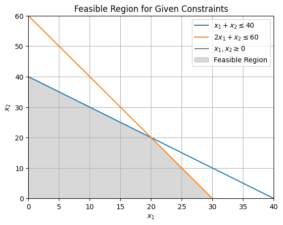
We can establish that the basic feasible solutions are equivalent to the corner point solutions by mapping resultant \(x_1, x_2\) values from the table onto the graph. Alternatively, we can establish that the corner point solutions are equivalent to the the basic feasible solutions by identifying each corner point to the corresponding set of non-basic variables.
Equivalently, in an \(n\)-dimensional space, the corner point of a feasible bounded region corresponds to a set of non-basic variables (and consequently basic variables). Hence, the fundamental idea behind the Simplex Algorithm is to evaluate all combinations of non-basic/basic variables, i.e. establish all corner points of the feasible region, compute objective function value for each, and thus determine the optimal solution.
For the given problem, we will thus have,
Non-Basic Variables |
Basic Variables |
Decision Variable \(\\(x_1, x_2)\) |
Slack Variable \(\\(s_1, s_2)\) |
Objective Function Value |
|---|---|---|---|---|
\(x_1, x_2\) |
\(s_1, s_2\) |
0, 0 |
40, 60 |
0 |
\(x_1, s_1\) |
\(x_2, s_2\) |
0, 40 |
0, 20 |
-60 |
\(x_2, s_2\) |
\(x_1, s_1\) |
30, 0 |
10, 0 |
-120 |
\(s_1, s_2\) |
\(x_1, x_2\) |
20, 20 |
0, 0 |
-140 |
Hence, the optimal value is \(x_1, x_2 = 20, 20\) rendering objective function value of \(z = -140\).
Now, we shall apply these concepts to solve a three dimensional linear optimisation problem.
Objective:
Subject to:
We begin by transforming the maximisation problem into a typical minimisation problem.
Objective:
Subject to:
We will now transform the above formulation into the standardised form by introducing a slack term into the technical constraints.
Objective:
Subject to:
Here, we have a system of 2 equations with 3 decision and 2 slack variables. Hence, we will set 3 variables as non-basic to evaluate the values for the remaining 2 as basic variables, and consequently compute the objective function value.
Non-Basic Variables |
Basic Variables |
Decision Variable \(\\(x_1, x_2. x_3)\) |
Slack Variable \(\\(s_1, s_2)\) |
Is Basic Feasible Solution? |
Objective Function Valuen |
|---|---|---|---|---|---|
\(x_1, x_2, x_3\) |
\(s_1, s_2\) |
0, 0, 0 |
8, 10 |
Yes |
0 |
\(x_1, x_2, s_1\) |
\(s_2, x_3\) |
- |
- |
No |
- |
\(x_1, x_2, s_2\) |
\(s_1, x_3\) |
0, 0, 10 |
8, 0 |
Yes |
-20 |
\(x_1, s_1, x_3\) |
\(s_2, x_2\) |
0, 8, 0 |
0, 10 |
Yes |
-16 |
\(x_1, s_2, x_3\) |
\(s_1, x_2\) |
- |
- |
No |
- |
\(s_1, x_2, x_3\) |
\(x_1, s_2\) |
4, 0, 0 |
0, 10 |
Yes |
-4 |
\(s_2, x_2, x_3\) |
\(x_1, s_1\) |
- |
- |
No |
- |
\(s_1, s_2, x_3\) |
\(x_1, x_2\) |
- |
- |
No |
- |
\(s_1, x_2, s_2\) |
\(x_1, x_3\) |
4, 0, 10 |
0, 0 |
Yes |
-24 |
\(x_1, s_1, s_2\) |
\(x_2, x_3\) |
0, 8, 10 |
0, 0 |
Yes |
-36 |
Thus, for the given 3 dimensional linear optimisation problem, the optimal value is \(x_1, x_2, x_3 = 0, 8, 10\) rendering objective function value of \(z = -36\).
Tip
The Simplex Algorithm
Step 1. Transform the \(n\)-dimensional linear optimisation problem with \(m\) technical constraints into the standardised form by introducing a slack term into each of the technical constraint. This should render a formulation with technical constraints represented by a system of \(m\) equations and \(n+m\) variables.
Step 2. Iterate through \((n+m)\) \(\text{C}\) \(m = (n+m)! / (n!m!)\) possible combinations of \(n\) non-basic variables and \(m\) basic variables to find the optimal solution
Step 2.1. Select \(n\) non-basic variables and set them to zero.
Step 2.2. Evaluate values for the \(m\) basic variables using \(m\) equations.
Step 2.3. Determine whether the set of basic/non-basic variables form a basic feasible solution. Recall, if the resulting values of basic variables satisfy \(\mathbf{x,s} \geq 0\), then the set of basic and non-basic variable values together \((\mathbf{x,s})\) are said to form a basic feasible solution.
Step 2.4 Repeat step 2.1. until all possible combinations of non-basic variables are set, else go to step 3.
Step 3. For all such basic feasible solution evaluate the objective function value and determine the optimal value.