
Lecture 25: Assignment 2 Discussion#
Multivariate Data Analysis & Vizualisation (11)
For the vehicles dataset from the fueleconomy package in R,
a. develop the following plots (10)
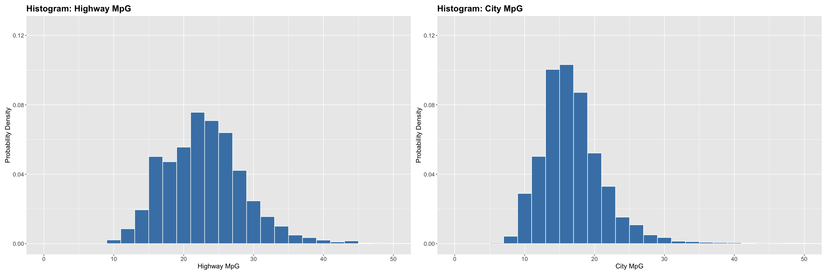
histogram for highway & city MpG
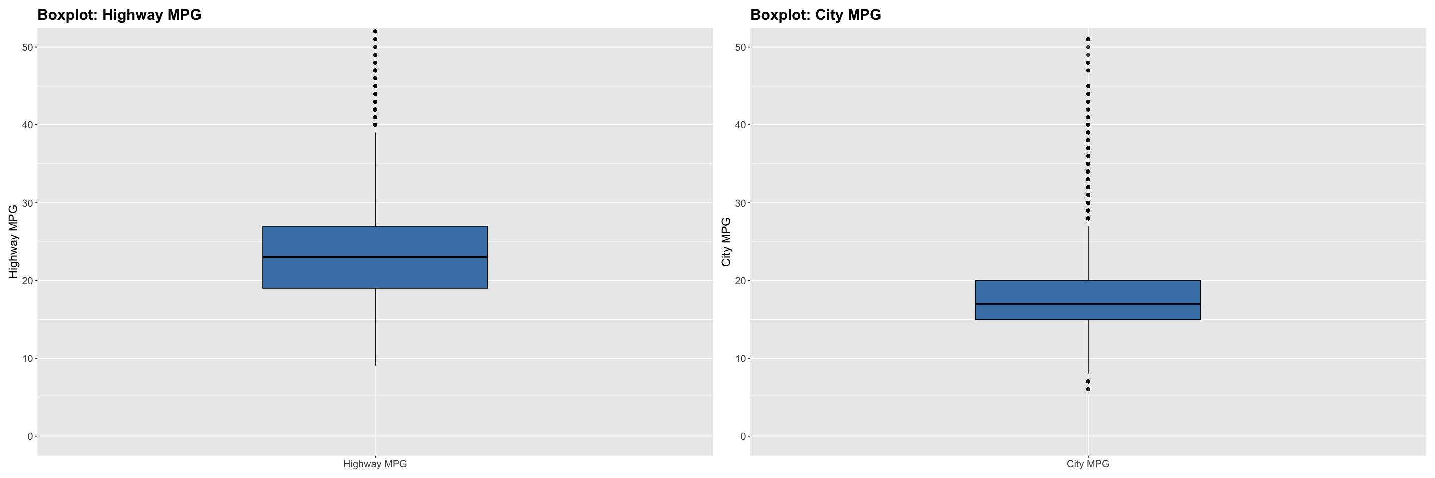
box plot for highway & city MpG
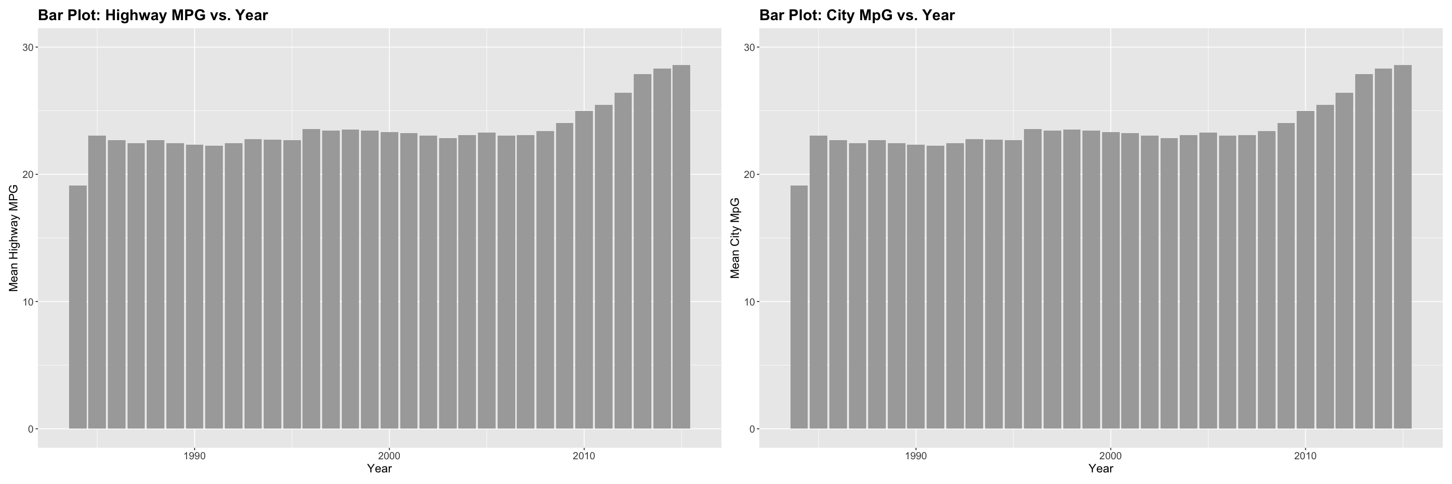
bar plot for mean highway & city MpG vs. vehicle year
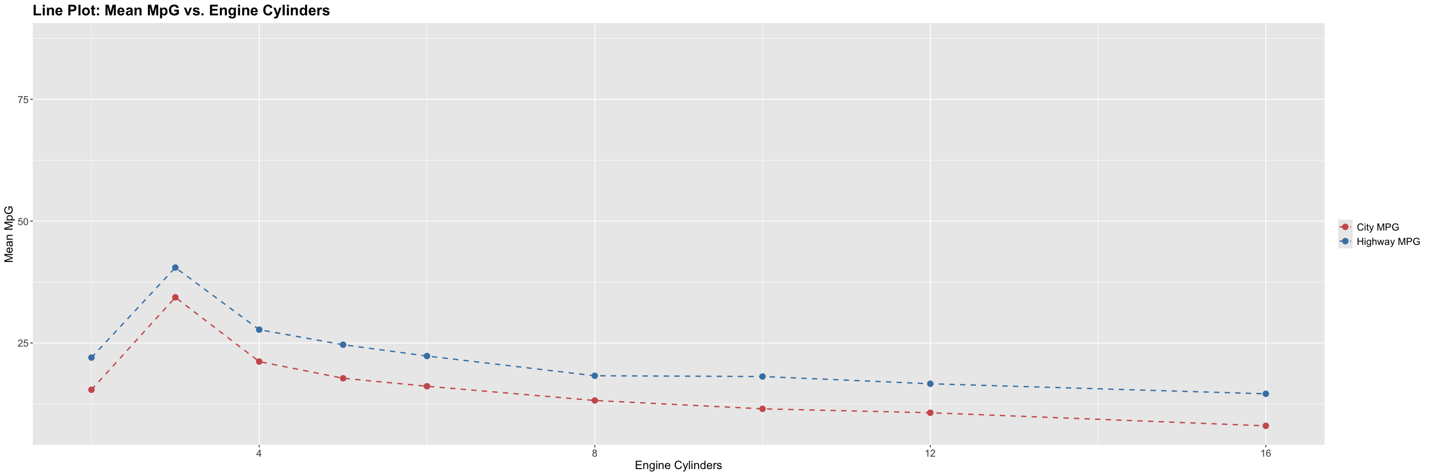
line plot for mean highway & city MpG vs. engine cylinders
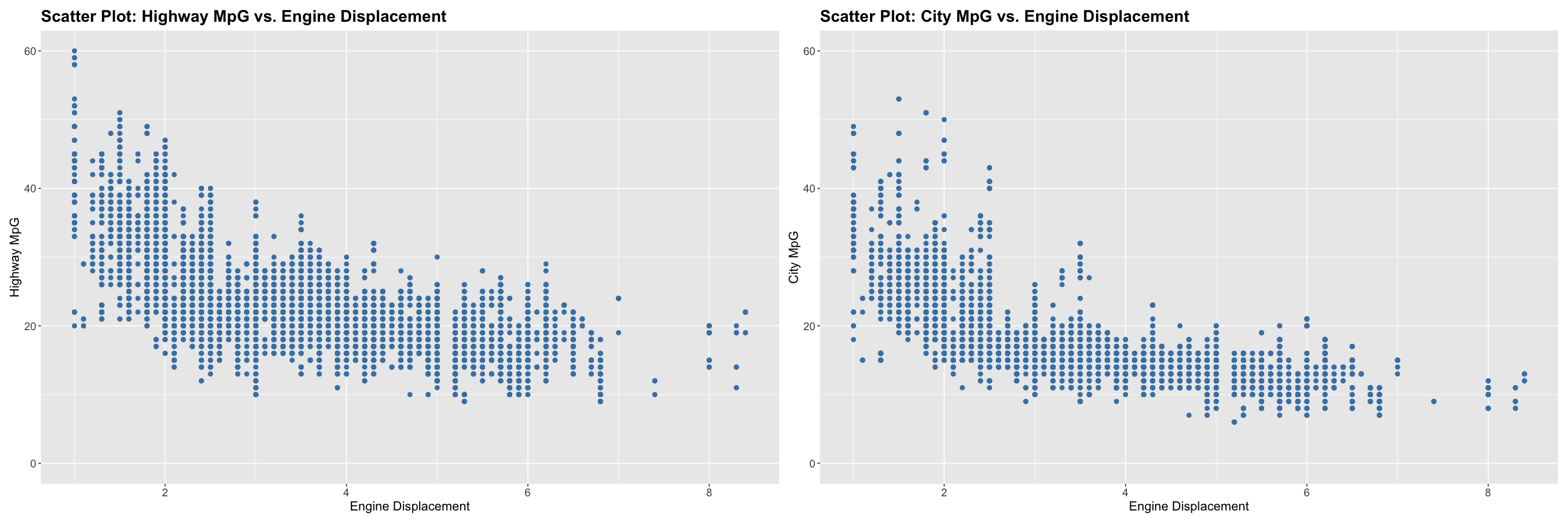
scatter plot for highway & city MpG vs. engine displacement
b. evaluate the correlation between (1)
engine displacement and highway & city MpG
engine cylinders and highway & city MpG
vehicle year and highway & city MpG
# Vehicles Dataset - Fuel Economy Package
## Load Packages
library(dplyr)
library(ggplot2)
library(patchwork)
library(fueleconomy)

# Load the dataset (filtered for non-zero & non-NA values; augmented with new variable 'I' indicating if vehicle is manufactured after 2009)
data <- fueleconomy::vehicles %>%
  filter(year != 0, cyl != 0, displ != 0, is.na(year) == FALSE, is.na(cyl) == FALSE, is.na(displ) == FALSE) %>%
  mutate(I = ifelse(year > 2009, 1, 0))
Attaching package: ‘dplyr’


The following objects are masked from ‘package:stats’:

    filter, lag


The following objects are masked from ‘package:base’:

    intersect, setdiff, setequal, union
options(repr.plot.width = 24, repr.plot.height = 8)

# Histograms for Highway MpG
p1 <- ggplot(data, aes(x = hwy, y = ..density..)) +
  geom_histogram(binwidth = 2, fill = "steelblue", color = "white") +
  labs(title = "Histogram: Highway MpG", x = "Highway MpG", y = "Probability Density") +
  coord_cartesian(xlim = c(0, 50), ylim = c(0, 0.125)) +
  theme(
    plot.title = element_text(size = 18, face = "bold"),
    axis.title = element_text(size = 14),
    axis.text  = element_text(size = 12),
    strip.text = element_text(size = 13, face = "bold")
  )

# Histograms for City MpG
p2 <- ggplot(data, aes(x = cty, y = ..density..)) +
  geom_histogram(binwidth = 2, fill = "steelblue", color = "white") +
  labs(title = "Histogram: City MpG", x = "City MpG", y = "Probability Density") +
  coord_cartesian(xlim = c(0, 50), ylim = c(0, 0.125)) +
  theme(
    plot.title = element_text(size = 18, face = "bold"),
    axis.title = element_text(size = 14),
    axis.text  = element_text(size = 12),
    strip.text = element_text(size = 13, face = "bold")
  )

# Combine the two histograms
p1 | p2
Warning message:
“The dot-dot notation (`..density..`) was deprecated in ggplot2 3.4.0.
ℹ Please use `after_stat(density)` instead.”
options(repr.plot.width = 24, repr.plot.height = 8)

# Boxplot for Highway MpG
p1 <- ggplot(data, aes(x = "Highway MPG", y = hwy)) +
  geom_boxplot(fill = "steelblue", color = "black", outlier.alpha = 0.7, width = 0.4) +
  labs(title = "Boxplot: Highway MPG", x = NULL, y = "Highway MPG") +
  coord_cartesian(ylim = c(0, 50)) +
  theme(
    plot.title = element_text(size = 18, face = "bold"),
    axis.title = element_text(size = 14),
    axis.text  = element_text(size = 12),
    strip.text = element_text(size = 13, face = "bold")
  )

# Boxplot for City MpG
p2 <- ggplot(data, aes(x = "City MPG", y = cty)) +
  geom_boxplot(fill = "steelblue", color = "black", outlier.alpha = 0.7, width = 0.4) +
  labs(title = "Boxplot: City MPG", x = NULL, y = "City MPG") +
  coord_cartesian(ylim = c(0, 50)) +
  theme(
    plot.title = element_text(size = 18, face = "bold"),
    axis.title = element_text(size = 14),
    axis.text  = element_text(size = 12),
    strip.text = element_text(size = 13, face = "bold")
  )

# Combine the two boxplots
p1 | p2
options(repr.plot.width = 24, repr.plot.height = 8)

# Prepare data
df <- fueleconomy::vehicles %>%
  group_by(year) %>%
  summarise(mean_hwy_mpg = mean(hwy), mean_cty_mpg = mean(cty))

# Create bar plots for mean highway and city MPG by year
p1 <- ggplot(df, aes(x = year)) +
  geom_bar(aes(y = mean_hwy_mpg), stat = "identity", position = "dodge", fill = "darkgrey") +
  labs(
    title = "Bar Plot: Highway MPG vs. Year",
    x = "Year",
    y = "Mean Highway MPG"
  ) +
  ylim(c(0, 30)) +
  theme(
    plot.title = element_text(size = 18, face = "bold"),
    plot.subtitle = element_text(size = 14),
    axis.title = element_text(size = 14),
    axis.text = element_text(size = 12)
  )

p2 <- ggplot(df, aes(x = year)) +
  geom_bar(aes(y = mean_hwy_mpg), stat = "identity", position = "dodge", fill = "darkgrey") +
  labs(
    title = "Bar Plot: City MpG vs. Year",
    x = "Year",
    y = "Mean City MpG"
  ) +
  ylim(c(0, 30)) +
  theme(
    plot.title = element_text(size = 18, face = "bold"),
    plot.subtitle = element_text(size = 14),
    axis.title = element_text(size = 14),
    axis.text = element_text(size = 12)
  )

# Combine the two bar plots
p1 | p2
options(repr.plot.width = 24, repr.plot.height = 8)

# Prepare data
df <- fueleconomy::vehicles %>%
  group_by(cyl) %>%
  summarise(mean_hwy_mpg = mean(hwy), mean_cty_mpg = mean(cty))

# Create a line plot for highway MpG and city MpG by engine cylinders
ggplot(df, aes(x = cyl)) +
  # Highway MPG
  geom_line(aes(y = mean_hwy_mpg, color = "Highway MPG", linetype = "Highway MPG"), linewidth = 0.75) +
  geom_point(aes(y = mean_hwy_mpg, color = "Highway MPG"), size = 3) +
  # City MPG
  geom_line(aes(y = mean_cty_mpg, color = "City MPG", linetype = "City MPG"), linewidth = 0.75) +
  geom_point(aes(y = mean_cty_mpg, color = "City MPG"), size = 3) +
  scale_color_manual(values = c("Highway MPG" = "steelblue", "City MPG" = "indianred")) +
  scale_linetype_manual(values = c("Highway MPG" = "dashed", "City MPG" = "dashed")) +
  labs(
    title = "Line Plot: Mean MpG vs. Engine Cylinders",
    x = "Engine Cylinders",
    y = "Mean MpG",
    color = NULL, linetype = NULL
  ) +
  theme(
    plot.title = element_text(size = 18, face = "bold"),
    axis.title = element_text(size = 14),
    axis.text  = element_text(size = 12),
    legend.text = element_text(size = 12)
  )
Warning message:
“Removed 1 row containing missing values or values outside the scale range
(`geom_line()`).”
Warning message:
“Removed 1 row containing missing values or values outside the scale range
(`geom_point()`).”
Warning message:
“Removed 1 row containing missing values or values outside the scale range
(`geom_line()`).”
Warning message:
“Removed 1 row containing missing values or values outside the scale range
(`geom_point()`).”
options(repr.plot.width = 24, repr.plot.height = 8)

# Scatter plot of highway MpG vs engine displacement
p1 <- ggplot(data, aes(x = displ, y = hwy)) +
  geom_point(color = "steelblue", size = 2) +
  labs(
    title = "Scatter Plot: Highway MpG vs. Engine Displacement",
    x = "Engine Displacement",
    y = "Highway MpG"
  ) +
  ylim(c(0, 60)) +
  theme(
    plot.title = element_text(size = 18, face = "bold"),
    plot.subtitle = element_text(size = 14),
    axis.title = element_text(size = 14),
    axis.text = element_text(size = 12)
  )

# Scatter plot of city MpG vs engine displacement
p2 <- ggplot(data, aes(x = displ, y = cty)) +
  geom_point(color = "steelblue", size = 2) +
  labs(
    title = "Scatter Plot: City MpG vs. Engine Displacement",
    x = "Engine Displacement",
    y = "City MpG"
  ) +
  ylim(c(0, 60)) +
  theme(
    plot.title = element_text(size = 18, face = "bold"),
    plot.subtitle = element_text(size = 14),
    axis.title = element_text(size = 14),
    axis.text = element_text(size = 12)
  )

# Combine the two scatter plots
p1 | p2
Warning message:
“Removed 1 row containing missing values or values outside the scale range
(`geom_point()`).”
# Correlation values
message("Correlation - Highway MpG vs. Vehicle Year         :   ", round(cor(data$hwy, data$year, use = "complete.obs"), digits = 3))
message("Correlation - City MpG vs. Vehicle Year            :   ", round(cor(data$cty, data$year, use = "complete.obs"), digits = 3))
message("Correlation - Highway MpG vs. Cylinder Count       :   ", round(cor(data$hwy, data$cyl, use = "complete.obs"), digits = 3))
message("Correlation - City MpG vs. Cylinder Count          :   ", round(cor(data$cty, data$cyl, use = "complete.obs"), digits = 3))
message("Correlation - Highway MpG vs. Engine Displacement  :   ", round(cor(data$hwy, data$displ, use = "complete.obs"), digits = 3))
message("Correlation - City MpG vs. Engine Displacement     :   ", round(cor(data$cty, data$displ, use = "complete.obs"), digits = 3))
Correlation - Highway MpG vs. Vehicle Year         :   0.208

Correlation - City MpG vs. Vehicle Year            :   0.097

Correlation - Highway MpG vs. Cylinder Count       :   -0.653

Correlation - City MpG vs. Cylinder Count          :   -0.712

Correlation - Highway MpG vs. Engine Displacement  :   -0.719

Correlation - City MpG vs. Engine Displacement     :   -0.748
Linear Regression (18)
For the vehicles dataset from the fueleconomy package in R,
a. develop the following models (5)
cty= \(\beta_0\) + \(\beta_1\)year+ \(\beta_2\)cyl+ \(\beta_3\)displhwy= \(\beta_0\) + \(\beta_1\)year+ \(\beta_2\)cyl+ \(\beta_3\)displ
b. for the two models, compute (6)
Sum of Squares Total (SST)
Sum of Squares Regression (SSR)
Sum of Squared Errors (SSE)
Residual Standard Error (RSE)
R-squared (\(R^2\))
Adjusted R-squared (\(\bar{R}^2\))
c. for the two models, (7)
develop residuals plot
comment upon the validity of the assumptions of linear regression
(Hint: To comment upon multicollinearity, develop pairwise correlation for the exogneous variables)
# Model
model_hwy <- lm(hwy ~ year + cyl + displ, data = data)
model_cty <- lm(cty ~ year + cyl + displ, data = data)

# Summary
cat("\nHighway MpG Model Statistics:\n")
summary(model_hwy)
cat("\nCity MpG Model Statistics:\n")
summary(model_cty)

# Statistics
cat("\nHighway MpG Model Statistics:\n")
sst <- sum((data$hwy - mean(data$hwy))^2)
ssr <- sum((model_hwy$fitted.values - mean(data$hwy))^2)
sse <- sum((data$hwy - model_hwy$fitted.values)^2)
rse <- sqrt(sse / (nrow(data) - 2))
Rsquared <- ssr / sst
AdjRsquared <- 1 - (1 - Rsquared) * (nrow(data) - 1) / (nrow(data) - 2)
cat(" SST               :", round(sst, 2), "\n")
cat(" SSR               :", round(ssr, 2), "\n")
cat(" SSE               :", round(sse, 2), "\n")
cat(" RSE               :", round(rse, 2), "\n")
cat(" R-squared         :", round(Rsquared, 3), "\n")
cat(" Adjusted R-squared:", round(AdjRsquared, 3), "\n")

cat("\nCity MpG Model Statistics:\n")
sst <- sum((data$cty - mean(data$cty))^2)
ssr <- sum((model_cty$fitted.values - mean(data$cty))^2)
sse <- sum((data$cty - model_cty$fitted.values)^2)
rse <- sqrt(sse / (nrow(data) - 2))
Rsquared <- ssr / sst
AdjRsquared <- 1 - (1 - Rsquared) * (nrow(data) - 1) / (nrow(data) - 2)
cat(" SST               :", round(sst, 2), "\n")
cat(" SSR               :", round(ssr, 2), "\n")
cat(" SSE               :", round(sse, 2), "\n")
cat(" RSE               :", round(rse, 2), "\n")
cat(" R-squared         :", round(Rsquared, 3), "\n")
cat(" Adjusted R-squared:", round(AdjRsquared, 3), "\n")

# Residuals Plot
options(repr.plot.width = 24, repr.plot.height = 8)
df <- data.frame(
  fitted = fitted(model_hwy),
  resid  = residuals(model_hwy)
)
p1 <- ggplot(df, aes(x = fitted(model_hwy), y = resid(model_hwy))) +
  geom_point(color = "steelblue", size = 2) +
  labs(
    title = "Residuals Plot: Highway MpG Model",
    x = "Fitted Values",
    y = "Error"
  ) +
  theme(
    plot.title = element_text(size = 18, face = "bold"),
    axis.title = element_text(size = 14),
    axis.text = element_text(size = 12)
  )
df <- data.frame(
  fitted = fitted(model_cty),
  resid  = residuals(model_cty)
)
p2 <- ggplot(df, aes(x = fitted(model_cty), y = resid(model_cty))) +
  geom_point(color = "steelblue", size = 2) +
  labs(
    title = "Residuals Plot: City MpG Model",
    x = "Fitted Values",
    y = "Error"
  ) +
  theme(
    plot.title = element_text(size = 18, face = "bold"),
    axis.title = element_text(size = 14),
    axis.text = element_text(size = 12)
  )

# Combine the two residuals plots
p1 | p2
Highway MpG Model Statistics:
Call:
lm(formula = hwy ~ year + cyl + displ, data = data)

Residuals:
     Min       1Q   Median       3Q      Max
-13.3742  -2.2852  -0.3742   1.8763  30.0925

Coefficients:
              Estimate Std. Error t value Pr(>|t|)
(Intercept) -281.75784    4.34952  -64.78   <2e-16 ***
year           0.15819    0.00218   72.56   <2e-16 ***
cyl           -0.33852    0.02681  -12.63   <2e-16 ***
displ         -2.70517    0.03419  -79.12   <2e-16 ***
---
Signif. codes:  0 ‘***’ 0.001 ‘**’ 0.01 ‘*’ 0.05 ‘.’ 0.1 ‘ ’ 1

Residual standard error: 3.699 on 33377 degrees of freedom
Multiple R-squared:  0.5826,	Adjusted R-squared:  0.5826
F-statistic: 1.553e+04 on 3 and 33377 DF,  p-value: < 2.2e-16
City MpG Model Statistics:
Call:
lm(formula = cty ~ year + cyl + displ, data = data)

Residuals:
    Min      1Q  Median      3Q     Max
-8.5171 -1.6947 -0.4210  0.9798 30.1391

Coefficients:
              Estimate Std. Error t value Pr(>|t|)
(Intercept) -1.272e+02  3.443e+00  -36.94   <2e-16 ***
year         7.721e-02  1.725e-03   44.74   <2e-16 ***
cyl         -6.549e-01  2.122e-02  -30.86   <2e-16 ***
displ       -1.799e+00  2.706e-02  -66.47   <2e-16 ***
---
Signif. codes:  0 ‘***’ 0.001 ‘**’ 0.01 ‘*’ 0.05 ‘.’ 0.1 ‘ ’ 1

Residual standard error: 2.928 on 33377 degrees of freedom
Multiple R-squared:  0.5917,	Adjusted R-squared:  0.5916
F-statistic: 1.612e+04 on 3 and 33377 DF,  p-value: < 2.2e-16
Highway MpG Model Statistics:
 SST               : 1094157
 SSR               : 637444.2
 SSE               : 456713.2
 RSE               : 3.7
 R-squared         : 0.583
 Adjusted R-squared: 0.583

City MpG Model Statistics:
 SST               : 700678.6
 SSR               : 414567.2
 SSE               : 286111.5
 RSE               : 2.93
 R-squared         : 0.592
 Adjusted R-squared: 0.592
message("Correlation - X1 vs. X2: ", round(cor(data$year, data$cyl, use = "complete.obs"), digits = 3))
message("Correlation - X2 vs. X3: ", round(cor(data$cyl, data$displ, use = "complete.obs"), digits = 3))
message("Correlation - X3 vs. X1: ", round(cor(data$displ, data$year, use = "complete.obs"), digits = 3))
Correlation - X1 vs. X2: 0.108

Correlation - X2 vs. X3: 0.899

Correlation - X3 vs. X1: 0.063
For both models,
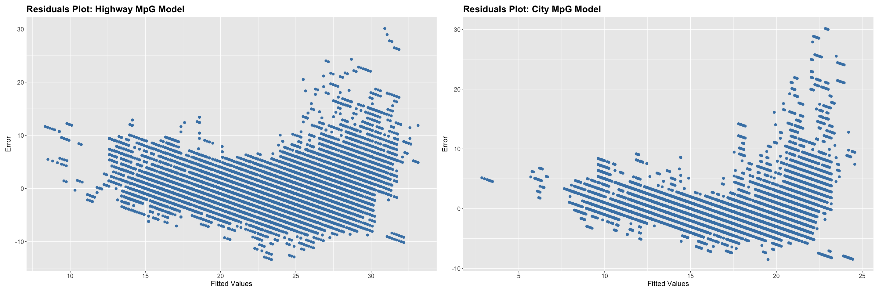
Linearity: Violated – The residuals also show a systematic curved pattern, indicating model misspecification or omitted nonlinear terms. Consequently, the estimates are no longer unbiased.
Independence: Satisfied – Given that the vehicle observations are independent (i.e., each vehicle is a distinct data point and not repeated measures), this assumption holds.
Homoskedasticity: Violated – The residuals plots exhibit a funnel like shape, indicating heteroskedasticity. Consequently, the estimates are no longer efficient.
No Multicollinearity: Violated – Number of engine cylinders is highly correlated with engine displacement. Consequently, the model is no longer interpretable.
Zero Conditional Mean of Errors: Violated – The curvature of the residuals plot, combined with its heteroskedastic nature, indicates that the error term is related to the predictor(s), again pointing towards model misspecification. Consequently, the estimates are no longer unbiased.
Symbolic Regression (5)
For the vehicles dataset from the fueleconomy package in R, compare the following models explored via symbolic regression with the linear regression model developed in the previous question (5)
cty= \(\beta_0\) + \(\beta_1\) \(\text{I}(\)year\(\geq 2010)\) + \(\beta_2\) \(\text{log}(\)displ\()\)hwy= \(\beta_0\) + \(\beta_1\) \(\text{I}(\)year\(\geq 2010)\) + \(\beta_2\) \(\text{log}(\)displ\()\)
(Hint: Compare the two set of models using model statistics and residual plots)
# Model
model_hwy <- lm(hwy ~ I + log(displ), data = data)
model_cty <- lm(cty ~ I + log(displ), data = data)

# Summary
cat("\nHighway MpG Model Statistics:\n")
summary(model_hwy)
cat("\nCity MpG Model Statistics:\n")
summary(model_cty)

# Statistics
cat("\nHighway MpG Model Statistics:\n")
sst <- sum((data$hwy - mean(data$hwy))^2)
ssr <- sum((model_hwy$fitted.values - mean(data$hwy))^2)
sse <- sum((data$hwy - model_hwy$fitted.values)^2)
rse <- sqrt(sse / (nrow(data) - 2))
Rsquared <- ssr / sst
AdjRsquared <- 1 - (1 - Rsquared) * (nrow(data) - 1) / (nrow(data) - 2)
cat(" SST               :", round(sst, 2), "\n")
cat(" SSR               :", round(ssr, 2), "\n")
cat(" SSE               :", round(sse, 2), "\n")
cat(" RSE               :", round(rse, 2), "\n")
cat(" R-squared         :", round(Rsquared, 3), "\n")
cat(" Adjusted R-squared:", round(AdjRsquared, 3), "\n")

cat("\nCity MpG Model Statistics:\n")
sst <- sum((data$cty - mean(data$cty))^2)
ssr <- sum((model_cty$fitted.values - mean(data$cty))^2)
sse <- sum((data$cty - model_cty$fitted.values)^2)
rse <- sqrt(sse / (nrow(data) - 2))
Rsquared <- ssr / sst
AdjRsquared <- 1 - (1 - Rsquared) * (nrow(data) - 1) / (nrow(data) - 2)
cat(" SST               :", round(sst, 2), "\n")
cat(" SSR               :", round(ssr, 2), "\n")
cat(" SSE               :", round(sse, 2), "\n")
cat(" RSE               :", round(rse, 2), "\n")
cat(" R-squared         :", round(Rsquared, 3), "\n")
cat(" Adjusted R-squared:", round(AdjRsquared, 3), "\n")

# Residuals Plot
options(repr.plot.width = 24, repr.plot.height = 8)
df <- data.frame(
  fitted = fitted(model_hwy),
  resid  = residuals(model_hwy)
)
p1 <- ggplot(df, aes(x = fitted(model_hwy), y = resid(model_hwy))) +
  geom_point(color = "steelblue", size = 2) +
  labs(
    title = "Residuals Plot: Highway MpG Model",
    x = "Fitted Values",
    y = "Error"
  ) +
  theme(
    plot.title = element_text(size = 18, face = "bold"),
    axis.title = element_text(size = 14),
    axis.text = element_text(size = 12)
  )
df <- data.frame(
  fitted = fitted(model_cty),
  resid  = residuals(model_cty)
)
p2 <- ggplot(df, aes(x = fitted(model_cty), y = resid(model_cty))) +
  geom_point(color = "steelblue", size = 2) +
  labs(
    title = "Residuals Plot: City MpG Model",
    x = "Fitted Values",
    y = "Error"
  ) +
  theme(
    plot.title = element_text(size = 18, face = "bold"),
    axis.title = element_text(size = 14),
    axis.text = element_text(size = 12)
  )

# Combine the two residuals plots
p1 | p2
Highway MpG Model Statistics:
Call:
lm(formula = hwy ~ I + log(displ), data = data)

Residuals:
     Min       1Q   Median       3Q      Max
-14.6933  -2.2845  -0.1289   1.9822  26.3067

Coefficients:
             Estimate Std. Error t value Pr(>|t|)
(Intercept)  34.69327    0.05665  612.45   <2e-16 ***
I             3.75479    0.05017   74.85   <2e-16 ***
log(displ)  -10.55936    0.04683 -225.49   <2e-16 ***
---
Signif. codes:  0 ‘***’ 0.001 ‘**’ 0.01 ‘*’ 0.05 ‘.’ 0.1 ‘ ’ 1

Residual standard error: 3.508 on 33378 degrees of freedom
Multiple R-squared:  0.6247,	Adjusted R-squared:  0.6247
F-statistic: 2.778e+04 on 2 and 33378 DF,  p-value: < 2.2e-16
City MpG Model Statistics:
Call:
lm(formula = cty ~ I + log(displ), data = data)

Residuals:
     Min       1Q   Median       3Q      Max
-11.1836  -1.5089  -0.2024   1.0190  27.2311

Coefficients:
            Estimate Std. Error t value Pr(>|t|)
(Intercept) 27.03649    0.04239  637.82   <2e-16 ***
I            2.36073    0.03754   62.89   <2e-16 ***
log(displ)  -8.94851    0.03504 -255.36   <2e-16 ***
---
Signif. codes:  0 ‘***’ 0.001 ‘**’ 0.01 ‘*’ 0.05 ‘.’ 0.1 ‘ ’ 1

Residual standard error: 2.625 on 33378 degrees of freedom
Multiple R-squared:  0.6718,	Adjusted R-squared:  0.6718
F-statistic: 3.416e+04 on 2 and 33378 DF,  p-value: < 2.2e-16
Highway MpG Model Statistics:
 SST               : 1094157
 SSR               : 683494.7
 SSE               : 410662.7
 RSE               : 3.51
 R-squared         : 0.625
 Adjusted R-squared: 0.625

City MpG Model Statistics:
 SST               : 700678.6
 SSR               : 470727.3
 SSE               : 229951.3
 RSE               : 2.62
 R-squared         : 0.672
 Adjusted R-squared: 0.672
message("Correlation - X1 vs. X2: ", round(cor(data$I, log(data$displ)), digits = 3))
Correlation - X1 vs. X2: 0.028
For both models,
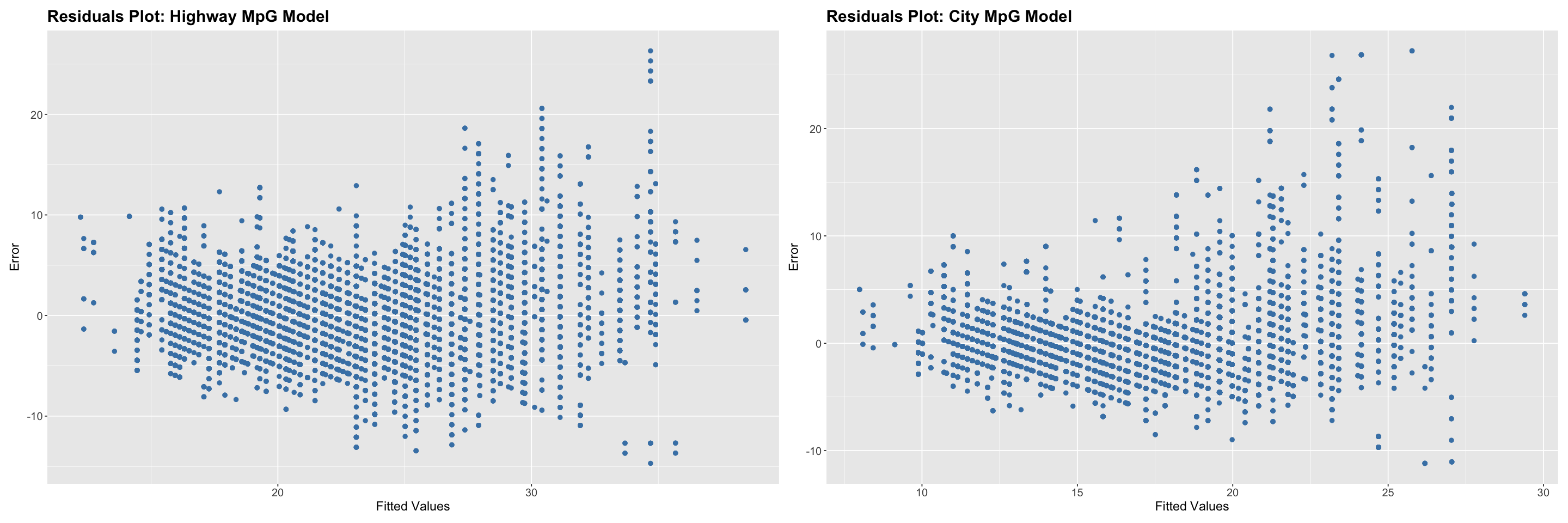
Linearity: Fairly Satisfied – The residuals do not exhibit a strong systematic curved pattern. Consequently, the estimates are likely unbiased.
Independence: Satisfied – Given that the vehicle observations are independent (i.e., each vehicle is a distinct data point and not repeated measures), this assumption holds.
Homoskedasticity: Violated – The residuals plots exhibit a funnel like shape, indicating heteroskedasticity. Consequently, the estimates are no longer efficient.
No Multicollinearity: Satisfied – The model exhibits low correlation between exogneous variable. Consequently, the model is interpretable.
Zero Conditional Mean of Errors: Fairly Satisfied – The residuals appear to be fairly centered around zero with no systematic pattern, supporting the assumption that the expected value of errors given the explanatory variable is zero. Consequently, the estimates are unbiased.
Logistic Regression (11)
For the TravelMode dataset from the AER. package in R, explore how alternate-specific variables (travel: in-vehicle travel time, wait: terminal waiting time, vcost: vehicle operational cost, and gcost: generalized travel cost) as well as individual-specific variables (income: household income, and size: traveling party size) impact choice of travel mode (air, train, bus, car). To this end,
(Note: The data is availble in long format with one row per individual–mode combination.)
a. develop the model (4)
b. compute the following statistics (7)
log-likelihood for the
equally likely model
market share model
estimated model
estimated model R-squared with respect to the
equally-likely model
market share model
estimated model adjusted R-squared with respect to the
equally-likely model
market share model
# TravelMode Dataset - AER Package
## Load Packages
library(AER)
library(dplyr)
library(mlogit)

## Load the dataset (choices mutated from yes/no to TRUE/FALSE)
data("TravelMode", package = "AER")
long_data <- TravelMode %>%
  mutate(choice = choice == "yes")

model_data <- mlogit.data(
  long_data,
  choice = "choice",
  shape = "long",
  chid.var = "individual",
  alt.var = "mode"
)
# Estimated Model
model <- mlogit(
  formula = choice ~ travel + wait + vcost + gcost | income + size,
  data = model_data,
  reflevel = "car"
)
summary(model)

# Model Statistics
I      <- max(as.integer(as.factor(long_data$individual))  )
J      <- length(unique(long_data$mode))
K      <- length(coef(model))
Y      <- long_data$choice
Z      <- long_data %>%
            filter(choice==TRUE) %>%
            count(mode, name = "n") %>%
            mutate(p = n / sum(n))
P      <- Z$p[model_data$alt]
LL_EL  <- sum(Y * log(1/J))
LL_MS  <- sum(Y * log(P))
LL_MNL <- as.numeric(logLik(model))
R2_EL  <- 1 - (LL_MNL / LL_EL)
R2_MS  <- 1 - (LL_MNL / LL_MS)
AR2_EL <- 1 - ((LL_MNL - K) / LL_EL)
AR2_MS <- 1 - ((LL_MNL - K) / LL_MS)

cat("\n--- Log-likelihoods ---\n")
cat(sprintf("EL  : %0.3f\n", LL_EL))
cat(sprintf("MS  : %0.3f\n", LL_MS))
cat(sprintf("MNL : %0.3f\n", LL_MNL))
cat("\n--- McFadden R^2 ---\n")
cat(sprintf("R2 vs EL : %0.4f\n", R2_EL))
cat(sprintf("R2 vs MS : %0.4f\n", R2_MS))
cat("\n--- Adjusted McFadden R^2 ---\n")
cat(sprintf("Adj R2 vs EL : %0.4f (K = %d)\n", AR2_EL, K))
cat(sprintf("Adj R2 vs MS : %0.4f (K = %d)\n", AR2_MS, K))
Call:
mlogit(formula = choice ~ travel + wait + vcost + gcost | income +
    size, data = model_data, reflevel = "car", method = "nr")

Frequencies of alternatives:choice
    car     air   train     bus
0.28095 0.27619 0.30000 0.14286

nr method
5 iterations, 0h:0m:0s
g'(-H)^-1g = 3.48E-07
gradient close to zero

Coefficients :
                    Estimate Std. Error z-value  Pr(>|z|)
(Intercept):air    5.2865000  1.2026299  4.3958 1.104e-05 ***
(Intercept):train  5.7082954  0.7266516  7.8556 3.997e-15 ***
(Intercept):bus    4.7163288  0.8238724  5.7246 1.037e-08 ***
travel            -0.0102498  0.0034179 -2.9988   0.00271 **
wait              -0.1025547  0.0113755 -9.0154 < 2.2e-16 ***
vcost             -0.0533528  0.0252825 -2.1103   0.03484 *
gcost              0.0464263  0.0249000  1.8645   0.06225 .
income:air         0.0080781  0.0134186  0.6020   0.54717
income:train      -0.0594981  0.0148925 -3.9952 6.465e-05 ***
income:bus        -0.0199412  0.0163648 -1.2185   0.22302
size:air          -0.5307014  0.3210340 -1.6531   0.09831 .
size:train         0.1628226  0.2394588  0.6800   0.49653
size:bus          -0.2399000  0.3580260 -0.6701   0.50282
---
Signif. codes:  0 ‘***’ 0.001 ‘**’ 0.01 ‘*’ 0.05 ‘.’ 0.1 ‘ ’ 1

Log-Likelihood: -170.69
McFadden R^2:  0.39848
Likelihood ratio test : chisq = 226.14 (p.value = < 2.22e-16)
--- Log-likelihoods ---
EL  : -291.122
MS  : -283.759
MNL : -170.688

--- McFadden R^2 ---
R2 vs EL : 0.4137
R2 vs MS : 0.3985

--- Adjusted McFadden R^2 ---
Adj R2 vs EL : 0.3690 (K = 13)
Adj R2 vs MS : 0.3527 (K = 13)