Lecture 31: Single-Server Queueing Systems

Note

This lecture details how to simulate a single-server queueing system laying foundations for multi-server queueing systems such as a Highway Toll Plaza. To this end, this lecture defines the problem and susbequently presents an example.

---

Problem Definition

Consider a single-server queueing system initialized empty and idle \(\left(t = 0, j = 0 \ \text{and} \ \varphi = 0 \right)\). A customer \(i\) arrving at inter-arrival time \(a_i\), either waits in the queue if the server is busy \(\left(\varphi = 1 \right)\), incurring a delay of \(d_i\), or directly enters service spanning a duration of \(s_i\), if the server is idle. Note, here we assume customer inter-arrival and service times to be independently, identically, and randomly distributed.

Figure: Illustration of a single-server queueing system

For this server, we are interested in the assessing following three performance metrics over a service of \(n\) customers spanning a total duration of \(t(n)\):

• Average Customer Delay: \(d(n) = \sum_{i=1}^n d_i / n\)

• Average Queue Length: \(q(n) = \sum_{j=1}^{\infty} jt_j / t(n)\), where \(t_j\) is the duration for which queue length is \(j\)

• Average Server Utilization: \(u(n) = \)t_{\varphi = 1} / t(n)\(, where \)t_{\varphi = 1}$ is the duration for which the server is busy

Note, these performance metrics represent outcomes of a single simulation. Hence, to comprehensively assess this server, we evaluate measures of location, dispersion, and shape on the performance metrics across a large number of simulations.

Note

While customer inter-arrival and service times are independently, idenitically, and randomly distirbuted random variables, customer delay, queue length, and server status are not. Specifically, these random variables, and consequently, average customer delay, average queue length, as well as average server utilization depend on the actual realisation of customer inter-arrival and service times.

Example

Consider a single-server queueing system with following inter-arrival times and service times.

\[\begin{split} A = [0.4, 1.2, 0.5, 1.7, 0.2, 1.6, 0.2, 1.4, 1.9] \\ S = [2.0, 0.7, 0.2, 1.1, 3.7, 0.6, 1.0, 1.0, 1.0] \end{split}\]

Simulate the system to calculate the average customer delay, average queue length, and average server utilization for 6 customers serviced by the server.

To do so, we begin by evaluating the arrival time for customer \(i\) using the interarrival times as follows: \(t^a_i = \sum^i_{k=1} a_k\), rendering,

\[ T_a = [0.4, 1.6, 2.1, 3.8, 4.0, 5.6, 5.8, 7.2, 9.1] \]

Subsequently, we evaluate the service start time for customer \(i\) based on queue length and server status. Specifically, customer \(i\) either waits in the queue if the server is busy, or directly enters service if the server is idle.

\[ T_s = [0.4, 2.4, 3.1, 3.8, 4.9, 8.6, 9.2, 10.2, 11.2] \]

Conseqeuntly, the delay observed by customer \(i\) is given as: \(d_i = t^s_i - t^a_i\), rendering

\[ D = [0.0, 0.8, 1.0, 0.0, 0.9, 3.0, 3.4, 3.0, 2.1] \]

Finally, the service end time is given by: \(t^i = t^s_i + s_i\) ,

\[ T_e = [2.4, 3.1, 3.3, 4.9, 8.6, 9.2, 10.2, 11.2, 12.2] \]

Combining the arrival, service start, and service end events, we get the following event clock \(T_o\):

\[ T_o = [0, 0.4, 0.4, 1.6, 2.1, 2.4, 2.4, 3.1, 3.1, 3.3, 3.8, 3.8, 4.0, 4.9, 5.6, 5.8, 7.2, 8.6, 8.6, 9.1, 9.2, 9.2, 10.2, 10.2, 11.2, 11.2] \]

At each point in time, we observed the following events:

\[ E = [o, a, s, a, a, e, s, e, s, e, a, s, a, e, s, a, a, a, e, s, a, e, s, e, s, e, s] \]

Considering the following event routine:

\[\begin{split} \begin{aligned} a & : & j & \gets j + 1 & ; & \ \ \varphi \gets \varphi \\ s & : & j & \gets j - 1 & ; & \ \ \varphi \gets 1 \\ e & : & j & \gets j & ; & \ \ \varphi \gets 0 \end{aligned} \end{split}\]

We can determine the queue length at each time stamp,

\[ J = [0, 1, 0, 1, 2, 2, 1, 1, 0, 0, 1, 0, 1, 1, 0, 1, 2, 3, 3, 2, 3, 3, 2, 2, 1, 1, 0] \]

This renders the following graph for queue length vs time,

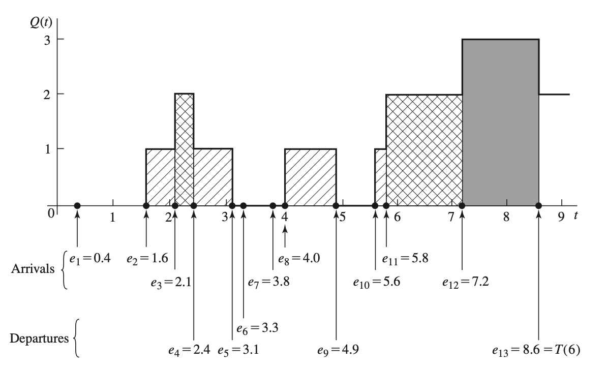
Figure: queue length, arrival times, and departure times for a realization of a single-server queueing system

Similarly, we can determine the server status at each time stamp,

\[ J = [0, 0, 1, 1, 1, 0, 1, 0, 1, 0, 0, 1, 1, 0, 1, 1, 1, 1, 0, 1, 1, 0, 1, 0, 1, 0, 1] \]

This renders the following graph for server status,

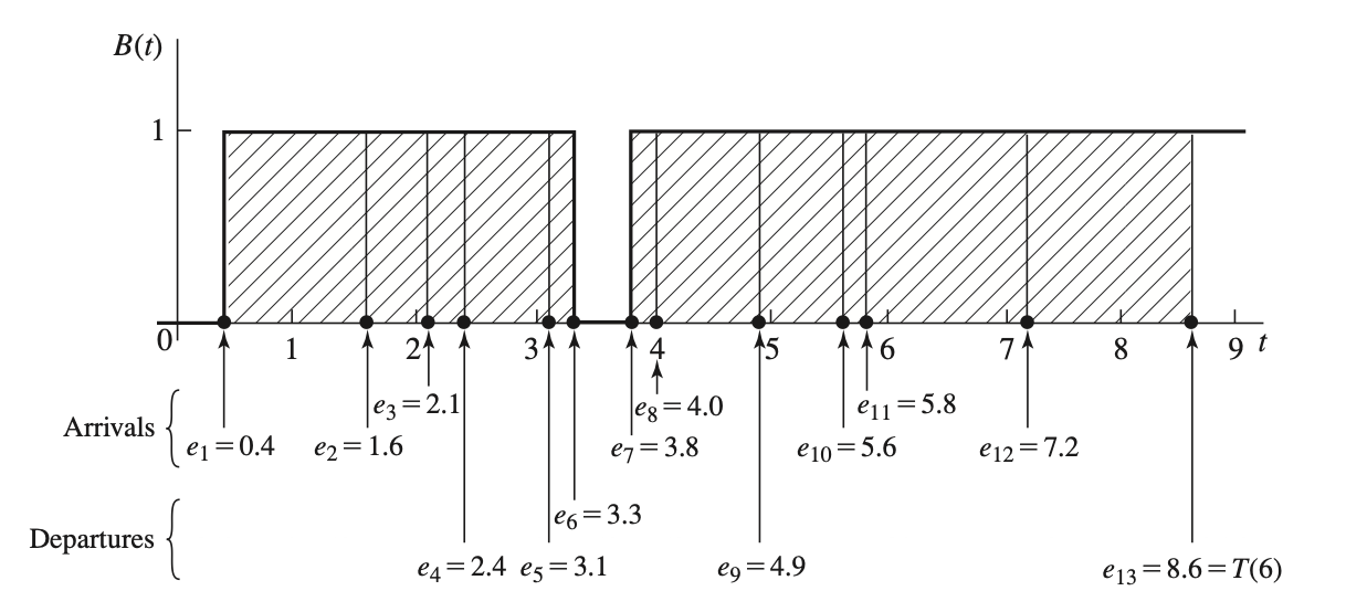
Figure: server utilization, arrival times, and departure times for a realization of a single-server queueing system.

For this simulation of the single server system we evaluate the the performance metrics, i.e, average delay, average queue length, and average utilization.

\[\begin{split} d(6) = 0.950 \\ q(6) = 1.217 \\ u(6) = 0.902 \\ \end{split}\]

Warning

For any simulation, we typically avoid measuing performance at the boundary conditions (warmup and cooldown). Thus, in the example demonstrated in this lecture, we ignore cooldown phase (customers 7-9). Note, we could have also ignored performance from the warmup phase (customers 1-3).

---

Note

In the next lecture, we will develop the simulation logic along with its implemenation in Python.