Lecture 1: Data

Note

This course introduces you to the science of drawing conclusions from data. To this end, this introduction lecture introduces a taxonomy of data along with tools for summarizing and visualizing data.

---

Taxonomy of Data

Data is a collection of observations of some quantity, quality, or category of some entity. For instance,

Entity	Quantitative	Qualitative	Categorical
Temperature	celsius	pleasant/unpleasant	hot/cold
Population Density	persons/sq.km.	low/high	rural/urban
Age	years	young/old	gen-z/millenial/gen-x/boomer/silent
Weight	kg	under-/over-weight	-
Height	cm	short/tall	-
Family Size	number of people	small/large	-
Biological Sex	-	-	male/female
Place of Birth	-	-	TN/RJ/WB/DL/…
Religion	-	-	hinduism/islam/christianity/…

Tip

The distinction between qualitative and categorical can sometimes be blurry. Generally, if there is an implicit ordering of the values the variable can take here is a tendency to call a variable qualitative rather than categorical.

Warning

During data collection or eventually at data analysis stage, one may code certain qualitiative/categorical variables as numerical values. For instance, height can be coded as short - 0 and tall - 1; or age group can be represented as gen-z - 0, millenial - 1, gen-x - 2, boomer - 3, and silent - 4. Despite this recoding, the inherent nature of the entity remains the same.

The quantitative entities can be further categorised as discrete and continuous. Specifically, the discrete quantitiative entities are countables on-hand, while continuous quantitiative entities cannot be hand-counted. For instance, age in years is a discrete quantitiative entity, while height in precise cms is a continuous quantitiative entity.

---

Test Yourself

1. How would you classify data collected on eye-colour of new-born babies at a hospital?

Discrete Quantitative
Continuous Quantitative
Qualitative
Categorical

2. How would you classify data collected on annual rainfall in inches?

Discrete Quantitative
Continuous Quantitative
Qualitative
Categorical

3. How would you classify data collected on GDP per capita rounded of to the nearest $ value?

Discrete Quantitative
Continuous Quantitative
Qualitative
Categorical

---

To showcase the process of summarizing and visualizing data, we shall use the 2024 Indian Time Use Survey (ITUS).

Note

A Time Use Survey, as the name suggests, is a systematic record of how individuals allocate their time across various activities over the course of a day. It captures detailed information on the duration, type, and context of each activity—such as working, commuting, household chores, leisure, caregiving, and personal care—typically over a 24-hour period. By documenting these daily routines, time use surveys provide valuable insights into patterns of labor participation (both paid and unpaid), gender roles, economic productivity, social engagement, and lifestyle behaviors within a population.

Summarizing Data

# 2024 ITUS Individual Data (original)
url  <- "https://raw.githubusercontent.com/anmpahwa/CE5540/refs/heads/main/resources/ITUS_IND_OG.csv"
data <- read.csv(url) # Loading Data
str(data)             # Data Structure

'data.frame':	533719 obs. of  23 variables:
 $ survey_year      : int  2024 2024 2024 2024 2024 2024 2024 2024 2024 2024 ...
 $ fsu_serial_no    : int  30010 30010 30010 30010 30010 30010 30010 30010 30010 30010 ...
 $ sector           : int  1 1 1 1 1 1 1 1 1 1 ...
 $ nss_region       : int  241 241 241 241 241 241 241 241 241 241 ...
 $ district         : int  17 17 17 17 17 17 17 17 17 17 ...
 $ stratum          : int  13 13 13 13 13 13 13 13 13 13 ...
 $ sub_stratum      : int  11 11 11 11 11 11 11 11 11 11 ...
 $ sub_round        : int  2 2 2 2 2 2 2 2 2 2 ...
 $ fod_sub_region   : int  2420 2420 2420 2420 2420 2420 2420 2420 2420 2420 ...
 $ nsc              : int  4 4 4 4 4 4 4 4 4 4 ...
 $ household_id     : int  1 2 2 2 2 3 3 3 3 3 ...
 $ individual_id    : int  1 1 2 3 4 1 2 3 4 5 ...
 $ response_code    : int  1 1 1 1 99999 1 1 1 1 1 ...
 $ day_of_week      : int  2 3 3 3 99999 7 7 7 7 7 ...
 $ type_of_day      : int  1 1 1 1 99999 1 1 1 1 1 ...
 $ relation_to_head : int  1 1 2 4 6 1 2 5 5 5 ...
 $ gender           : int  1 1 2 2 1 1 2 1 1 2 ...
 $ age              : int  45 54 52 29 3 48 44 23 13 18 ...
 $ marital_status   : int  1 2 2 2 1 2 2 1 1 1 ...
 $ education_level  : int  10 6 4 10 1 5 2 5 4 4 ...
 $ employment_status: int  10 94 92 31 99999 51 92 11 91 92 ...
 $ industry         : int  85 99999 99999 86 99999 1 99999 1 99999 99999 ...
 $ weight           : num  208857 208857 208857 208857 208857 ...

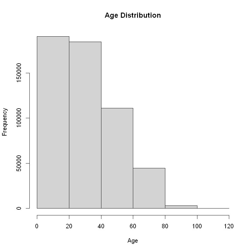
# Summarizing Age
message("Summary of Age")
message("     Min         : ", round(min(data$age), 2))
message("     1st Quartile: ", round(quantile(data$age, 0.25), 2))
message("     Median      : ", round(median(data$age), 2))
message("     Mean        : ", round(mean(data$age), 2))
message("     3rd Quartile: ", round(quantile(data$age, 0.75), 2))
message("     Max         : ", round(max(data$age), 2))

Summary of Age

     Min         : 0

     1st Quartile: 13

     Median      : 29

     Mean        : 30.42

     3rd Quartile: 45

     Max         : 118

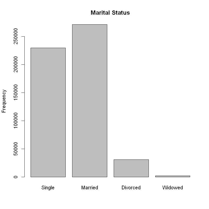
# Summarizing Marital Status
message("Summary of Marital Status")
message("     Single  : ", sum(data$marital_status == 1))
message("     Married : ", sum(data$marital_status == 2))
message("     Divorced: ", sum(data$marital_status == 3))
message("     Widowed : ", sum(data$marital_status == 4))

Summary of Marital Status

     Single  : 229274

     Married : 271056

     Divorced: 31071

     Widowed : 2318

Visualizing Data

hist(data$age,
     main = "Age Distribution",
     xlab = "Age",
     ylab = "Frequency",
     breaks = 5)

barplot(table(factor(data$marital_status, levels = 1:4, labels = c("Single", "Married", "Divorced", "Widowed"))),
        main = "Marital Status",
        ylab = "Frequency")

---

Tip

In addition to the above stated taxonomy discussed in this lecture, data can also be classified on temporal basis (static vs. dynamic) and certainty basis (deterministic vs. stochastic).