import matplotlib
if not hasattr(matplotlib.RcParams, "_get"):
    matplotlib.RcParams._get = dict.get
Lecture 27: Setting up Python#
Note
Python is an open-source, high-level, general-purpose programming language known for its simplicity and readability. Originally developed by Guido van Rossum in the late 1980s and first released in 1991, Python has since grown into one of the most popular programming languages for data analysis, machine learning, web development, automation, and scientific computing. Its strength lies in its extensive standard library, vibrant ecosystem of third-party packages, and ability to integrate seamlessly with other languages and tools.
Installing Python and JupyterLab / VS Code on Windows#
Follow these steps:
Step 1: Install Python#
Visit the official Python website: https://www.python.org/downloads/.
Download the latest stable version of Python (e.g., 3.x series) for Windows.
Run the installer:
Important: Check the box “Add Python to PATH” before clicking Install Now.
This ensures that Python commands can be run from the terminal.
Verify installation:
Open Command Prompt and type:
python --version
Step 2: Install VS Code#
Visit the official Visual Studio Code website: https://code.visualstudio.com/.
Download the Windows installer and run it.
During installation:
Select the option to add “Open with Code” to the right-click context menu.
Optionally, allow adding VS Code to the system PATH.
Launch VS Code after installation.
Step 3: Install the Python Extension for VS Code#
Open VS Code.
Go to the Extensions view (click the square icon on the left sidebar or press Ctrl+Shift+X).
Search for Python and install the extension published by Microsoft.
This extension adds syntax highlighting, IntelliSense, debugging, and Jupyter Notebook support.
Step 4: Install JupyterLab (Optional but Recommended)#
Open Command Prompt or VS Code Terminal and type:
pip install jupyterlabLaunch JupyterLab by typing:
jupyter lab
Once installed, open VS Code to begin writing Python code!
# Hello World in R
print("Hello World!")
Hello World!
Data Types in Python#
Python supports the following basic data types:
Character
Numeric
Integer
Logical
Complex
Here are some examples:
# Character
x = "CE5540"
print("Type of x is: ", type(x))

# Float
r = 3.14
print("Type of y is: ", type(r))

# Integer
v = int(42)
print("Type of v is: ", type(v))

# Logical
f = True
print("Type of f is: ", type(f))

# Complex
z = 2 + 3j
print("Type of z is: ", type(z))
Type of x is:  <class 'str'>
Type of y is:  <class 'float'>
Type of v is:  <class 'int'>
Type of f is:  <class 'bool'>
Type of z is:  <class 'complex'>
Data Structures in Python#
Python supports the following data structures:
Vectors
Matrices
Lists
Data Frames
Here are some examples:
import numpy as np
import pandas as pd

# Vectors
v1 = ["Apple", "Banana", "Mango"]
v2 = [9, 1, 5, 4, 6, 7, 0, 3, 8]
v3 = list(range(1, 6))  # R's 1:5
print("# Vectors")
print(v1)
print(v2)
print(v3)
print(f"Accessing a value in a vector: v1[0] = {v1[0]}. \nNotice that Python uses 0-based indexing!")

# Matrices (NumPy arrays)
data = [9, 1, 5, 4, 6, 7, 0, 3, 8]
## By row
m1 = np.array(data).reshape(3, 3, order='C')
## By column
m2 = np.array(data).reshape(3, 3, order='F')
print("\n# Matrices")
print("m1 (by row):\n", m1)
print("m2 (by column):\n", m2)
print(f"Accessing a value in a matrix: m1[0, 2] = {m1[0, 2]}")

# Dictionaries
l = {"name": "John", "age": 25, "scores": [90, 85, 88]}
print("\n# Dict")
print(l)
print(f"Accessing a value in a dict: l['name'] = {l['name']}")

# Data Frames (pandas)
df = pd.DataFrame({"Name": ["Alice", "Bob"], "Age": [23, 25]})
print("\n# Data Frame")
print(df)
print(f"Accessing a value in a data frame: df['Age'].iloc[0] = {df['Age'].iloc[0]}")
# Vectors
['Apple', 'Banana', 'Mango']
[9, 1, 5, 4, 6, 7, 0, 3, 8]
[1, 2, 3, 4, 5]
Accessing a value in a vector: v1[0] = Apple.
Notice that Python uses 0-based indexing!

# Matrices
m1 (by row):
 [[9 1 5]
 [4 6 7]
 [0 3 8]]
m2 (by column):
 [[9 4 0]
 [1 6 3]
 [5 7 8]]
Accessing a value in a matrix: m1[0, 2] = 5

# Dict
{'name': 'John', 'age': 25, 'scores': [90, 85, 88]}
Accessing a value in a dict: l['name'] = John

# Data Frame
    Name  Age
0  Alice   23
1    Bob   25
Accessing a value in a data frame: df['Age'].iloc[0] = 23
Control Flow#
Here is how you would write control flow statements in Python
x = 10

if x > 0:
    print("x is a positive number")
elif x < 0:
    print("x is a negative number")
else:
    print("x is zero!")
x is a positive number
Writing Loops in Python#
Python supports both for and while loops.
# For loop
print("# For Loop")
for i in range(1, 6):  # range(1, 6) generates 1, 2, 3, 4, 5
    print("Iteration:", i)

# While loop
print("\n\n# While Loop")
i = 1
while i <= 5:
    print("Count:", i)
    i = i + 1
# For Loop
Iteration: 1
Iteration: 2
Iteration: 3
Iteration: 4
Iteration: 5


# While Loop
Count: 1
Count: 2
Count: 3
Count: 4
Count: 5
Writing Functions in Python#
Functions are blocks of code that can be reused. Here’s how to define and call one.
# Factorial Function (Iterative Form)
def factorial_iterative(n):
    result = 1
    for i in range(2, n + 1):  # range is end-exclusive, so use n+1
        result *= i
    return result

# Example usage
print(factorial_iterative(5))  # Output: 120
120
# Factorial Function (Recursive Form)
def factorial_recursive(n):
    if n == 0 or n == 1:
        return 1
    else:
        return n * factorial_recursive(n - 1)

# Example usage
print(factorial_recursive(5))  # Output: 120
120
Summarising Data in Python#
In this segment of the lecture, we will develop measures of location, dispersion, and shape discussed in the previous lecture through 2024 ITUS sample individual dataset.
import pandas as pd

# 2024 ITUS Individual Data (original)
url  = "https://raw.githubusercontent.com/anmpahwa/CE5540/refs/heads/main/resources/ITUS_IND_OG.csv"
data = pd.read_csv(url)  # Loading Data

# Data structure
print(data.info())
<class 'pandas.core.frame.DataFrame'>
RangeIndex: 533719 entries, 0 to 533718
Data columns (total 23 columns):
 #   Column             Non-Null Count   Dtype
---  ------             --------------   -----
 0   survey_year        533719 non-null  int64
 1   fsu_serial_no      533719 non-null  int64
 2   sector             533719 non-null  int64
 3   nss_region         533719 non-null  int64
 4   district           533719 non-null  int64
 5   stratum            533719 non-null  int64
 6   sub_stratum        533719 non-null  int64
 7   sub_round          533719 non-null  int64
 8   fod_sub_region     533719 non-null  int64
 9   nsc                533719 non-null  int64
 10  household_id       533719 non-null  int64
 11  individual_id      533719 non-null  int64
 12  response_code      533719 non-null  int64
 13  day_of_week        533719 non-null  int64
 14  type_of_day        533719 non-null  int64
 15  relation_to_head   533719 non-null  int64
 16  gender             533719 non-null  int64
 17  age                533719 non-null  int64
 18  marital_status     533719 non-null  int64
 19  education_level    533719 non-null  int64
 20  employment_status  533719 non-null  int64
 21  industry           533719 non-null  int64
 22  weight             533719 non-null  float64
dtypes: float64(1), int64(22)
memory usage: 93.7 MB
None
# Filtering out into a smaller dataset
data = data[(data["nss_region"] == 241) & (data["employment_status"] == 81)]

# View the filtered data (head for preview)
print(data.head())
     survey_year  fsu_serial_no  sector  nss_region  district  stratum  \
38          2024          30010       1         241        17       13
210         2024          30013       1         241        26       13
225         2024          30013       1         241        26       13
229         2024          30013       1         241        26       13
312         2024          30014       1         241        29       13

     sub_stratum  sub_round  fod_sub_region  nsc  ...  day_of_week  \
38            11          2            2420    4  ...            1
210           10          1            2423    4  ...            4
225           10          1            2423    4  ...            7
229           10          1            2423    4  ...            7
312           11          4            2420    4  ...            7

     type_of_day  relation_to_head  gender  age  marital_status  \
38             1                 5       1   22               1
210            1                 5       1   18               1
225            1                 6       1   18               1
229            1                 5       1   19               1
312            1                 5       1   35               1

     education_level  employment_status  industry    weight
38                10                 81     99999  208857.0
210                5                 81     99999  207000.0
225                5                 81     99999  207000.0
229                4                 81     99999  207000.0
312                2                 81     99999  196571.0

[5 rows x 23 columns]
import pandas as pd
import numpy as np
from scipy import stats

# Measures of Location
z1 = data["age"].mean()     # Mean
z2 = data["age"].median()   # Median
z3 = data["age"].mode()[0]  # Mode (returns Series, take first)

print("Mean:", round(z1, ndigits=3))
print("Median:", round(z2, ndigits=3))
print("Mode:", round(z3, ndigits=3))

# Measures of Dispersion
z1 = data["age"].max() - data["age"].min()      # Range
z2 = stats.iqr(data["age"], nan_policy="omit")  # IQR
z3 = data["age"].std()                          # Standard deviation

print("Range:", round(z1, ndigits=3))
print("IQR:", round(z2, ndigits=3))
print("SD:", round(z3, ndigits=3))

# Measures of Distribution
z1 = stats.skew(data["age"], nan_policy="omit")     # Skewness
z2 = stats.kurtosis(data["age"], nan_policy="omit") # Kurtosis (Fisher's definition)

print("Skewness:", round(z1, ndigits=3))
print("Kurtosis:", round(z2, ndigits=3))
Mean: 26.949
Median: 23.0
Mode: 18
Range: 70
IQR: 11.0
SD: 11.423
Skewness: 1.816
Kurtosis: 4.337
Linear Regression in Python#
# Load necessary libraries
import pandas as pd
import seaborn as sns
import statsmodels.api as sm
import matplotlib.pyplot as plt

# Notebook/plot display options
plt.rcParams['figure.figsize'] = (9, 6)
pd.set_option('display.max_columns', None)  # Optional: show all columns when printing

# 2024 ITUS Individual Data (original)
url  = "https://raw.githubusercontent.com/anmpahwa/CE5540/refs/heads/main/resources/ITUS_HHD_DT.csv"
data = pd.read_csv(url)

# Data structure
print(data.info())
<class 'pandas.core.frame.DataFrame'>
RangeIndex: 139487 entries, 0 to 139486
Data columns (total 21 columns):
 #   Column               Non-Null Count   Dtype
---  ------               --------------   -----
 0   Unique_HH_ID         139487 non-null  object
 1   time_of_year         139487 non-null  int64
 2   day_of_week          139487 non-null  int64
 3   sector               139487 non-null  int64
 4   region               139487 non-null  int64
 5   district_population  139487 non-null  int64
 6   gender_ratio         139487 non-null  float64
 7   average_age          139487 non-null  float64
 8   marital_status       139487 non-null  int64
 9   highest_eduLevel     139487 non-null  int64
 10  employment_ratio     139487 non-null  float64
 11  family_structure     139487 non-null  float64
 12  household_size       139487 non-null  int64
 13  religion             139487 non-null  int64
 14  social_group         139487 non-null  int64
 15  land_possessed       139487 non-null  int64
 16  total_expenditure    139487 non-null  int64
 17  dwelling_unit        139487 non-null  int64
 18  dwelling_structure   139487 non-null  int64
 19  weight               139487 non-null  int64
 20  shopping_choice      139487 non-null  int64
dtypes: float64(4), int64(16), object(1)
memory usage: 22.3+ MB
None
Scatter Plot#
# Scatter Plot
plt.scatter(
    data["average_age"],
    np.log10(data["total_expenditure"] / data["household_size"]),
    color="steelblue",
    s=15  # matches your earlier size=2 in ggplot (Matplotlib uses points^2)
)
plt.title("Average Age vs Log Monthly Expenditure per Capita", fontsize=12, fontweight="bold")
plt.xlabel("Average Age", fontsize=10)
plt.ylabel("Log Monthly Expenditure per Capita", fontsize=10)
plt.xticks(fontsize=9)
plt.yticks(fontsize=9)

plt.show()
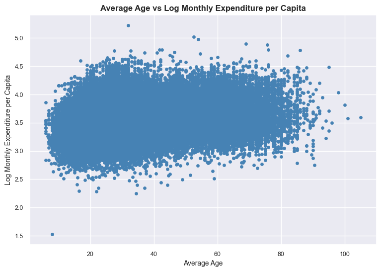
# Compute Pearson correlation
correlation = data["average_age"].corr(np.log10(data["total_expenditure"] / data["household_size"]))
print("Correlation between average age and monthly expenditure:", round(correlation, 3))
Correlation between average age and monthly expenditure: 0.264
# Define variables
X = data["average_age"]
y = np.log10(data["total_expenditure"] / data["household_size"])

# Fit linear regression model
X = sm.add_constant(X)
model = sm.OLS(y, X, missing="drop").fit()

# Display summary
print(model.summary())
                            OLS Regression Results
==============================================================================
Dep. Variable:                      y   R-squared:                       0.070
Model:                            OLS   Adj. R-squared:                  0.070
Method:                 Least Squares   F-statistic:                 1.047e+04
Date:                Sun, 10 Aug 2025   Prob (F-statistic):               0.00
Time:                        16:16:59   Log-Likelihood:                -1697.0
No. Observations:              139487   AIC:                             3398.
Df Residuals:                  139485   BIC:                             3418.
Df Model:                           1
Covariance Type:            nonrobust
===============================================================================
                  coef    std err          t      P>|t|      [0.025      0.975]
-------------------------------------------------------------------------------
const           3.3684      0.002   2060.789      0.000       3.365       3.372
average_age     0.0046   4.52e-05    102.317      0.000       0.005       0.005
==============================================================================
Omnibus:                     4880.760   Durbin-Watson:                   0.757
Prob(Omnibus):                  0.000   Jarque-Bera (JB):             6665.938
Skew:                           0.374   Prob(JB):                         0.00
Kurtosis:                       3.767   Cond. No.                         90.2
==============================================================================

Notes:
[1] Standard Errors assume that the covariance matrix of the errors is correctly specified.
# Errors

# Sums of squares
sst = np.sum((np.asarray(model.model.endog) - np.asarray(model.model.endog).mean())**2)             # total
ssr = np.sum((np.asarray(model.fittedvalues)  - np.asarray(model.model.endog).mean())**2)          # regression
sse = np.sum((np.asarray(model.model.endog) - np.asarray(model.fittedvalues))**2)                  # error

# Degrees of freedom
n = int(model.nobs)
p = int(model.df_model) + 1   # number of parameters incl. intercept
df_resid = int(model.df_resid)

# Metrics
rse = np.sqrt(sse / df_resid)
R2 = ssr / sst
AdjR2 = 1 - (1 - R2) * (n - 1) / (n - p)

print("SST               :", round(sst, 2))
print("SSR               :", round(ssr, 2))
print("SSE               :", round(sse, 2))
print("RSE               :", round(rse, 2))
print("R-squared         :", round(R2, 3))
print("Adjusted R-squared:", round(AdjR2, 3))
SST               : 8996.15
SSR               : 628.05
SSE               : 8368.1
RSE               : 0.24
R-squared         : 0.07
Adjusted R-squared: 0.07
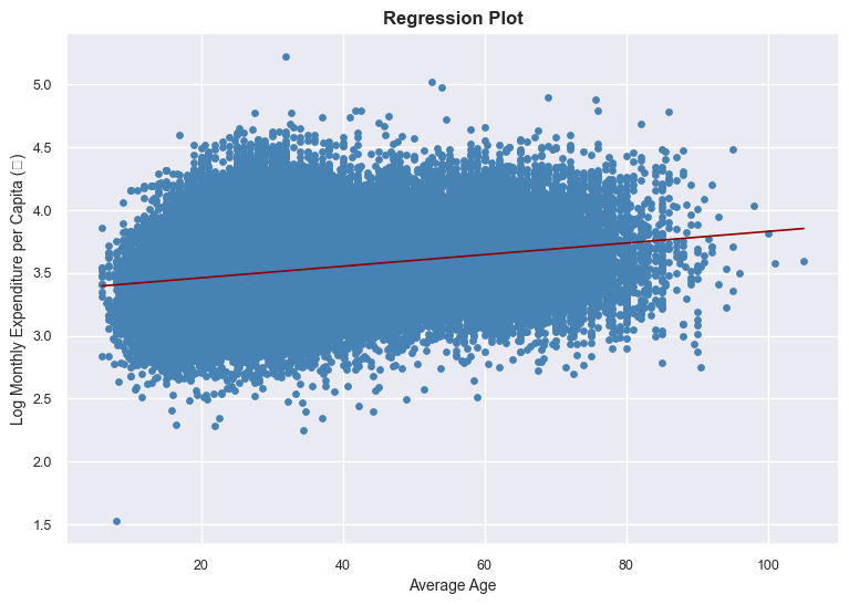
# Define variables
x = data["average_age"]
y = np.log10(data["total_expenditure"] / data["household_size"])

# Fit simple linear regression y = m*x + b
m, b = np.polyfit(x, y, 1)

# Regression line for plotting
x_line = np.linspace(x.min(), x.max(), 200)
y_line = m * x_line + b

# Scatter
plt.scatter(x, y, color="steelblue", s=15)

# Regression line (no CI, like se = FALSE)
plt.plot(x_line, y_line, color="darkred", linewidth=1.2)

# Labels & styling
plt.title("Regression Plot", fontsize=12, fontweight="bold")
plt.xlabel("Average Age", fontsize=10)
plt.ylabel("Log Monthly Expenditure per Capita (₹)", fontsize=10)
plt.xticks(fontsize=9)
plt.yticks(fontsize=9)

plt.show()
/Users/anmolpahwa/Library/Python/3.13/lib/python/site-packages/IPython/core/pylabtools.py:170: UserWarning: Glyph 8377 (\N{INDIAN RUPEE SIGN}) missing from font(s) Arial.
  fig.canvas.print_figure(bytes_io, **kw)
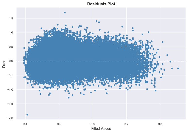
# Extract fitted values and residuals from statsmodels model
fitted_vals = model.fittedvalues
residuals = model.resid

# Scatter plot of residuals vs fitted values
plt.scatter(fitted_vals, residuals, color="steelblue", s=15)

# Add horizontal zero reference line
plt.axhline(y=0, color="black", linestyle="--", linewidth=0.8)

# Labels & styling
plt.title("Residuals Plot", fontsize=12, fontweight="bold")
plt.xlabel("Fitted Values", fontsize=10)
plt.ylabel("Error", fontsize=10)
plt.xticks(fontsize=9)
plt.yticks(fontsize=9)

plt.show()